2.1.2. Pipelining the data process

As the preferred language for artificial intelligence, Python is featured as its rich ecosystem, as well as the convenience for fast implementation and developing. Data processing involving in different technical approaches requires systematical integration. Thus, the unified data controlling among those utilities contributes to accelerate verifying prototypes, optimize algorithm performance, as well as lower maintenance cost.

Figure 2.2 ecosystem of Python

Data processing is akin to an assembly line, where an increase in the number of steps results in a exponential growth of factors that can impact the final result. While manually configuring all possible options for trial may seem feasible, it often leads to a chaotic outcome.

An uniform protocol, or programming norm, is therefore not only of advantages in integrating various tools developed by teams in different fields in Python ecosystem, but also time-saving for building practical pipelines or applications, on basis of each naive functional module. Following examples demonstrate how to establish pipelines for automating complex tasks.

2.1.2.1. Normalized scientific computing

Scientific computing flow implemented through informatics functions is of high completeness. And their units are readily to be flexibly reused when create new processing flow. Code 2.9 is a snippet in implementation for exporting Figure 2.9.

Code 2.9 flexibility and reusability of unit

u1, u2, u3, u4, u5, v1, v2 = [Unit(mappings=[_]) for _ in [load, binarize, identification_cells, colorize,
                                                           tsb.connected_domain, imshow, hist]]
to_fig1 = u1 >> v1
to_fig2 = u1 >> u2 >> v1
to_fig3 = Unit(mappings=[F(lambda **kw: [res := (u1 | (u1 >> u2 >> u3 >> u4))(**kw),
                                         np.dstack([res[1], np.linalg.norm(res[0], ord=2, axis=2)])][-1])]) >> v1
to_fig4 = Unit(mappings=[F(lambda **kw: np.array([_.sum() for _ in (u1 >> u2 >> u3 >> u5)(**kw)]))]) >> v2

to_fig3 corresponds to the case (c). Obtain this figure must overlap the random colored cell nucleus masks, superpositioned with grey scale image, then pass on an image viewer unit. It is the reason unit u1 is arranged paralleled with a sequential processing line u1 >> u2 >> u3 >> u4.

To export the (c) case in Figure 2.9, call to_fig3(data=file). If a researcher desires other parameters, call to_fig3(data=file, **user_defined_config). Or in more complicated situation, if the researcher want to compare outcomes from an identical pipe in different parameters, those derived pipes can also be readily obtained by: p = to_fig3.shadow(**config1) | to_fig3.shadow(**config2).

2.1.2.2. Automation experiment

There are also meta tools, for automation computing. The following example concerned the difference between global prewitt and canny filters on a natural image:

Code 2.10 auto experiment pipeline

from info.me import Unit, F
from info.me import tensorn as tsn
from info.vis import visualization as vis
from info.ins import datasets
import numpy as np
img = datasets.cat()

config = vis.FigConfigs.Histogram.update(width=1.2, name=['prewitt', 'canny'])
evaluate = F(lambda **kw: [res := kw.get('data'), print(np.std(res[0]-res[1])),
                           vis.Canvas.play(data=np.array([res[0].ravel(), res[1].ravel()]),
                                                          fig_type='histogram', cvs_legend=True,
                                                          fig_configs=config), res][-1])
u1, u2, u3, u4, u5, v1 = [Unit(mappings=[_]) for _ in [tsn.cropper, tsn.gaussian_filter, tsn.resize, tsn.prewitt_filter,
                                                       tsn.canny_filter, evaluate]]
p = u1 >> u2 >> u3 >> (u4 | u5) >> v1
p.required_args  # {'data', 'new_size', 'k_shape', 'crop_range'}

It includes data processing functions dealing with cropping, de-noising, and resampling, followed by another paralleled unit of filters. The user-customized process is implemented via lambda calculus: print out the standard deviation of difference between two paralleled output, display their pixel distribution difference, then return those two filtered figures.

As most functions in tensor namespace, including the F lambda, have been already registered as informatics version, the p can automatically analyze what keyword arguments are the required at least. Making a parameter pool based on the required arguments. The following code can auto trigger the experiments then dump each running case.

Code 2.11 run auto experiment

to_test = {
    'data': [img],
    'crop_range': [[(0.2, 0.2), (0.8, 0.8)], [(0.3, 0.3), (0.7, 0.7)]],
    'k_shape': [(3, 3), (6, 6), (9, 9)],
    'new_size': [(400, 400), (600, 600)]
}

from info.me import autotesting as tst
res = tst.experiments(data=p, params_pool=to_test, to_file='./experiment_results')

Prompt will info the current condition and calculated standard deviation, running time, and the final result case by case; then the histogram figure will be popped up like Figure 2.3.

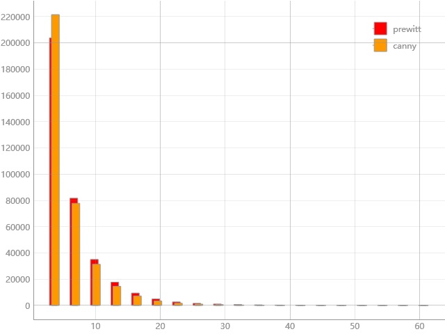
Figure 2.3 histogram for pixels distribution after prewitt and canny filters

All experiment results will be collected into a persistence file titled experiment_results.pyp inplace.

2.1.2.3. Automation testing

Different from automation experiment which can export the computed results, the automation testing only records the exit code. If the pipeline exits with raised exception, related information will also be noted. Similar as experiments in Code 2.11, this meta implementation funtest is in the same namespace. It can test for informatics functions, unit and pipelines defined via this framework.

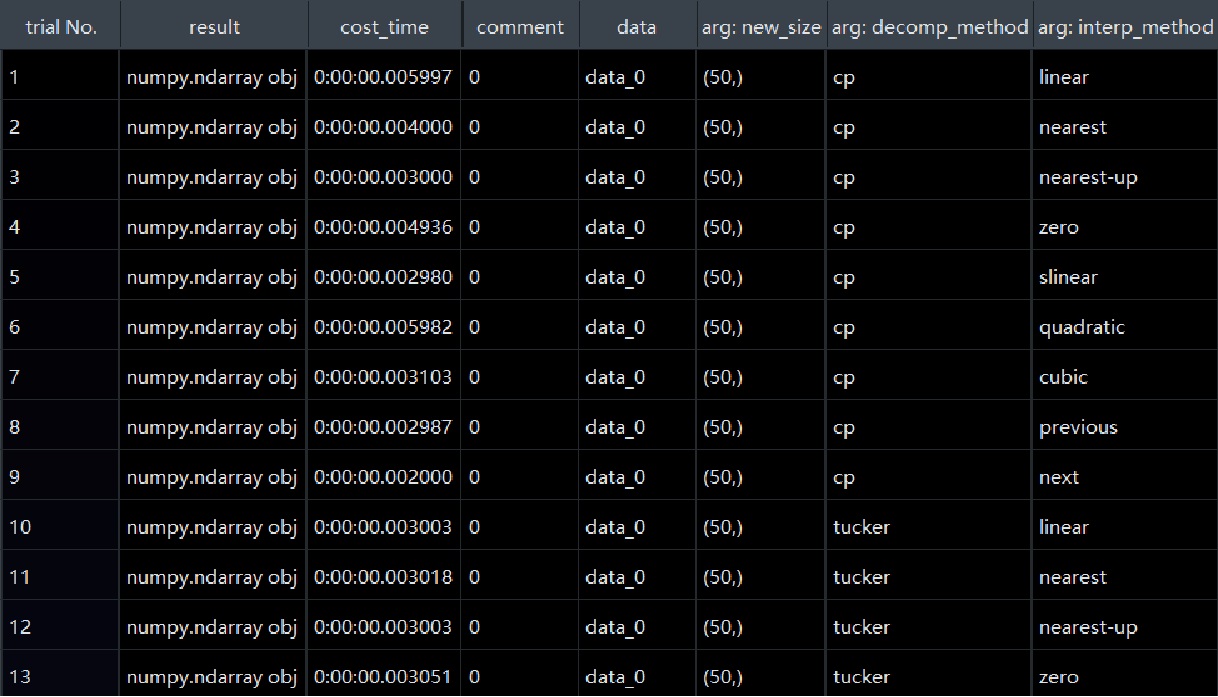
Figure 2.4 automation testing result for resize function

Figure 2.4 is the test result for resize function. Class type remains in result column. The cost time, arguments for each test item are also be recorded.

---

Authors:

Chen Zhang

Version:

0.0.5

Created on:

Feb 7, 2024