2.2.2. Data transform and identification

In data analytics, machine learning, or deep learning, approaches to build proper pipes of pre and post processing, are critical steps for determining the ceiling of model performance. Data defined here mainly refers to \(n\)-dimensional array in computer science (or tensor in mathematics). This tutorial demonstrates image enhancement methods generally applied in computer vision, as well as their upper applications in certain study fields.

2.2.2.1. Edge and corner detection

General filters can be applied on tensor for profile detection, keypoint identification for registration, and such like. Figure 2.5 reveal the effect of (b) the bilateral filter, (c) the canny filter and (d) the harris response, applied on (a) a original natural image, respectively. The edge of objects, as well as corner-like region can be emphasised through those data processing methods.

Different transformations might contribute for varying objectives: de-noising processing possibly prefers the bilateral filtered result; to evaluate degree of interspace of bricks, canny response would be helpful.

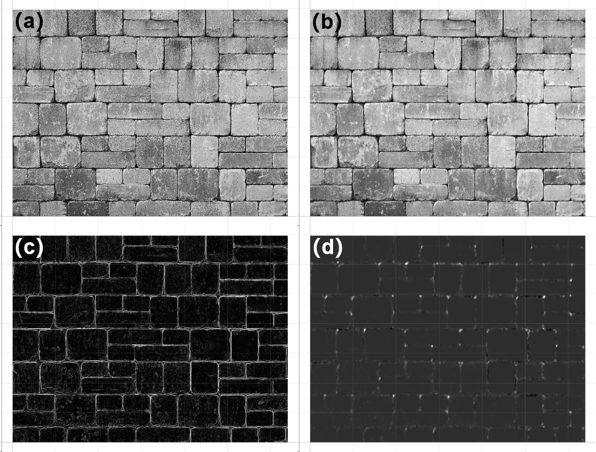
Figure 2.5 bilateral filter, edge and corner response

Additionally, those processing transforms can also be called, in consistence with data with different dimension(s). Figure 2.6 shows harris response for high curvature, on 1-dimensional series, and Figure 2.7 is canny filter applied on a 3-dimensional cubic instance.

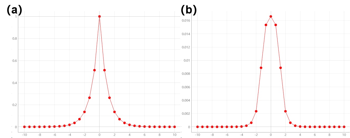
Figure 2.6 harris response on 1D series

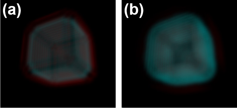
Figure 2.7 canny filter on 3D volume

Code 2.16 is for referenced implementation, as well as visualization for those examples.

Code 2.16 natural image processing

from info.me import tensorn as tsn
from info.vis import visualization as vis
from info.vis import ImageViewer
from info.ins import datasets
import numpy as np


img = datasets.bricks()
imgs = [img, tsn.bilateral_filter(data=img, k_shape=(5, 5)),
        tsn.canny_filter(data=img), tsn.harris_response(data=img, k_shape=(10, 10))]
for f in imgs:
    vis.Canvas.play(data=f, fig_type='image')

f1 = (lambda s: np.min(np.array([np.e ** s, np.e ** (-s)]), axis=0))
x = np.linspace(-10, 10, 31)
y = f1(x)
y1 = tsn.harris_response(data=y, k_shape=(4,))
vis.Canvas.play(data=(x, y))
vis.Canvas.play(data=(x, y1))


def cubic(r, c, shape=(50, 50, 40)):
    res = np.zeros(shape)
    for idx in np.argwhere(res == 0):
        if (r1 := np.linalg.norm(idx-c, ord=4)) < r:
            res[tuple(idx)] = r1
    return res * 50


s1 = cubic(7, np.array([25, 25, 20]))
s2 = tsn.canny_filter(data=s1)
ImageViewer.play(data=s1)
ImageViewer.play(data=s2)

With appropriate method of transformation customized for specific task as upstream processing, information with high analytical value remains while disturbance signal is restricted, therefore increasing upper bond on performance of modeling, can rationally be expected.

2.2.2.2. Segmentation for quantitative statistics

Quantitative analysis takes labeling different objects from a total segmentation as the prerequisite. In practice, some classic algorithms, or their combinations can be applied to identify each individual, then downstream mathematical statistics, as well as corresponding analysis are capable to be undertaken.

As illustrated in Figure 2.8, for determining each instance in condition that overlapped area among two or more might occur, proper configuration of distance transform combined with connected domain will precisely allocate each basin for initial flooding seed.

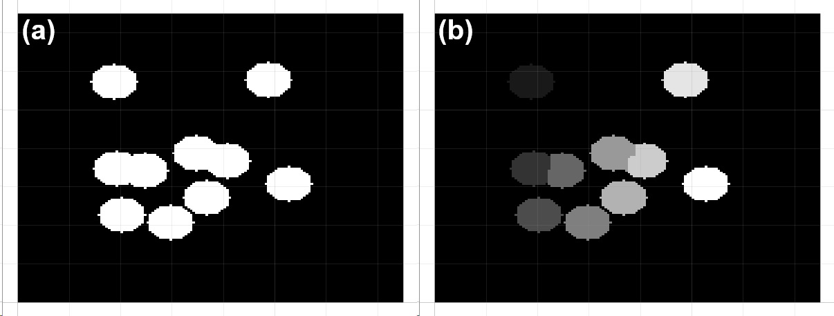
Figure 2.8 labeling segmentation through topography

Demonstrated implementation is as showed in Code 2.17:

Code 2.17 segmentation labeling

from info.me import tensorb as tsb
from info.vis import visualization as vis
from scipy.ndimage import distance_transform_edt
import numpy as np
np.random.seed(10)


msk = np.zeros((150, 150)).astype(bool)
msk[25:125, 25:125] = True
msk = np.sum([_ for _ in tsb.prober(data=msk, prob_nums=10, prob_radius=9)], axis=0).astype(bool)
vis.Canvas.play(data=msk, fig_type='image')
geo, seeds = -distance_transform_edt(msk), np.zeros_like(msk).astype(bool)
seeds[np.where(geo < -8)] = True
seeds = np.sum([(i+1)*e for i, e in enumerate(tsb.connected_domain(data=seeds))], axis=0)

# labeling with different integers:
res = tsb.watershed(data=msk, flood_seeds=seeds)
vis.Canvas.play(data=res, fig_type='image')

2.2.2.3. Data processing on different disciplines

Comprehensively utilizing those essential techniques for transform and identification, can build considerably complicated data processing pipelines on many study fields. Figure 2.9 is for evaluating equivalent area of tumor cell nucleus. Data is collected from a hepatocellular carcinoma case from The Cancer Genome Atlas (TCGA) program.

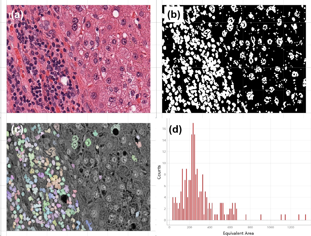
Figure 2.9 statistics for nucleus of tumor cells on pathological image

Another example is for surveying and mapping engineering. After certain preprocessing flows, road net can be highlighted, and the envelopes for water, grass, tree cover, and the corresponding area percentages were determined as well, as showed in Figure 2.10.

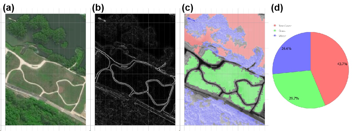
Figure 2.10 semantic statistics on topography

In material research, measuring grain is a conventional approach to understand formation, as well as the principle of the formation of microstructure. Figure 2.11 demonstrates grain boundaries determination via 2nd order differential transformation followed by labels identification, then exporting scatter plots for grain radius and area as x- and y-axis, respectively. The test data is from a bulletin published on Vac Aero.

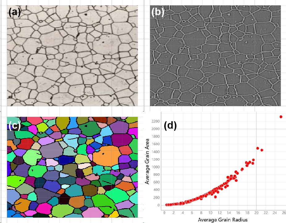
Figure 2.11 metallic grain measurement

---

Authors:

Chen Zhang

Version:

0.0.5

Created on:

Jan 2, 2024