4.3.1. Feature capturing

4.3.1.1. How we define features

In many field, people process and analysis data, not only for summary, but for the possible fact underneath the data self. Different disciplines have their own context or terminology. In machine learning, we call it pattern; in statistics, we call it probability distribution; in physics or other related researches, we call it model. However, when it comes to this concept, they consistently desires there’s the thing: the minimal representation of information.

Use the image recognition task for example, values of grey level varies pixel to pixel, but people can still distinguish the objective from background, can tell whether the object is a person, or the other creatures. Thus, even though pixel varies, the form of their combinations, or the location where they changed, is regular to some extent.

Concisely, the really informative thing is not pixels themselves, but how they distributed, where they changed. If the thing is capable enough to automatically finish a certain task, it can be considered as the features, bonding with this task.

4.3.1.2. Spatial filtering

Spatial filtering is the techniques to emphasis the local features. It is applied globally, but can augment local contrast where obvious changes occurs. This tech has been widely used in edge detection, object recognition.

The Figure 4.12 shows the principle of spatial filtering applied in 2 dimensional image. kernel moves globally on image, and values of output image are replaced pixel by pixel based on pre-defined computing method.

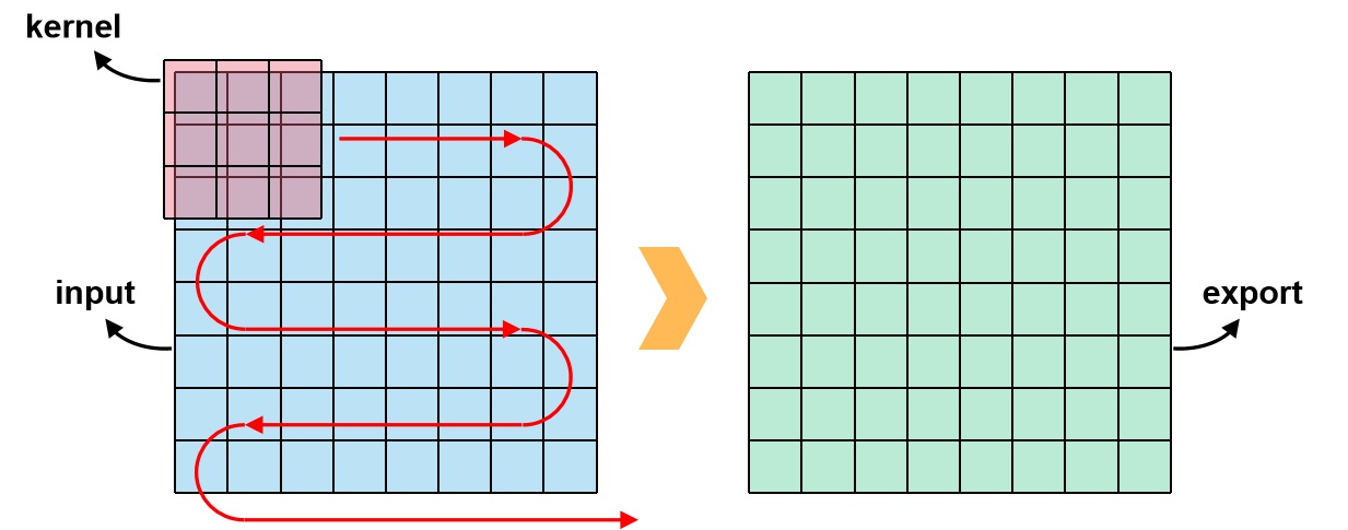
Figure 4.12 data transition via kernel

The most used computing methods, are illustrated in Figure 4.13. \(\boldsymbol{K}\) refers kernel, and the values from \(r\) to \(z\) are the weights in \(\boldsymbol{K}\). \(\boldsymbol{F}\) refers the figure, and the values from \(a\) to \(i\) are the numeric on \(\boldsymbol{F}\), overlapped where the kernel \(\boldsymbol{K}\) is currently located. \(\boldsymbol{I}\) is the numeric to replace after filtering. The difference between correlation and convolution, is the order of weight. Additionally, there also some generic filter using certain statistic on the localized values (e.g. rank filter).

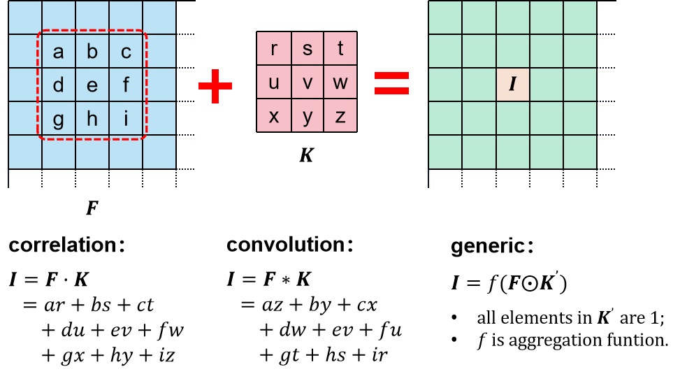
Figure 4.13 correlation, convolution, and generic mapping using kernel

Technically, it is not enough to understand how values will be calculated, but where the replacement will take place. There’s a concept of anchor in kernel, as shown in Figure 4.14. The grey pixel is the anchor location of kernel where the pixel will be replaced. By default, an anchor should be the center of a kernel (otherwise the output image will be biased), however, it is weired to limit all dimensions of kernel as odd numbers. The basic idea in scipy is showed in Figure 4.14 which is also applied in informatics, for even number, the anchor in that dimension will be located one pixel next to the center.

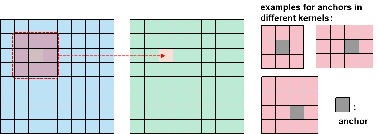
Figure 4.14 positions of anchor in kernels

In addition, when kernel moves on edges or corners of the image, the real numeric in original image will be insufficient for calculation. In this condition it requires padding some pseudo-data in outer scope. Figure 4.15 shows five padding methods. Keep in mind that this factor only makes difference on the corner- or edge-like regions.

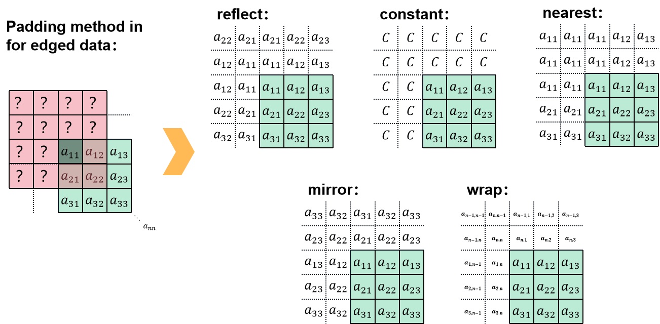
Figure 4.15 padding methods for numerical computing in edges

Back to the kernel itself. Different kernels are designed for different purposes. For example, gaussian kernel is a center-emphasising localized averaging, can be used for smoothing or de-noising. laplacian of gaussian kernel using contrary signs between center and the area enveloped, to measure the local contrast. The gaussian kernel and laplacian of gaussian kernel in 2 dimension are illustrated in Figure 4.16 and Figure 4.17.

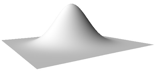
Figure 4.16 gaussian kernel

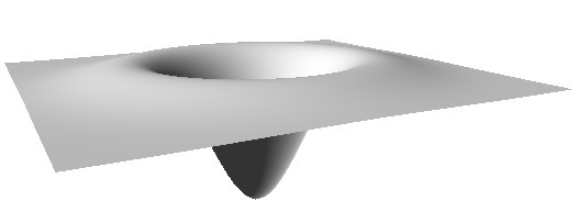
Figure 4.17 laplacian of gaussian kernel

The effect of denoising, or object edge and profile detection, through gaussian and some gaussian-related kernels filtering will be like:

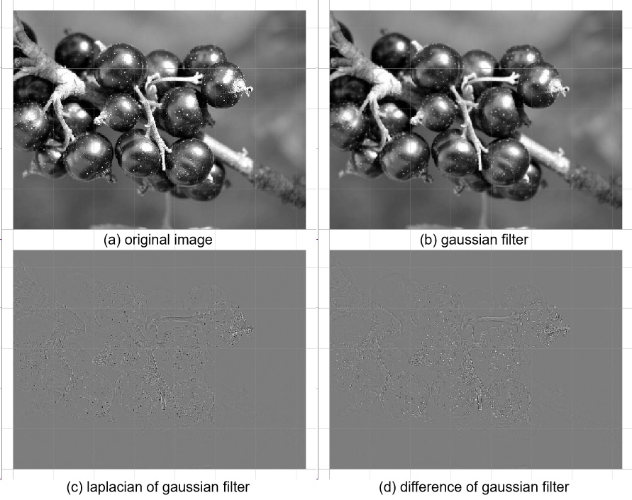
Figure 4.18 spatial filtering applied on image processing

Note

Most kernels are central symmetric, in which condition the correlation and convolution will be substantially equivalent.

Some kernels are designed to augment features along some certain orientations, due to their aeolotropy. For example, the real part of 2-dimensional gabor kernel with radian of \(\theta = 0.5\pi\) will be like the surface in Figure 4.19

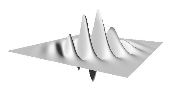
Figure 4.19 gabor kernel

Specifying the desired direction of spatial sine harmonic function, the texture of object aligned with, will be augmented. This tech is generally thought to be in accordance with the principle of primary visual cortex. It can be applied on feature engineering for data augmentation for multipurpose, if the directional information of the data is though to be of importance in analysis. For easy of understanding, here shows the real and imaginary parts of the case (a) in Figure 4.18 convolved using gabor filtering, with directions of \((1, 0)\) and \((0, 1)\), respectively:

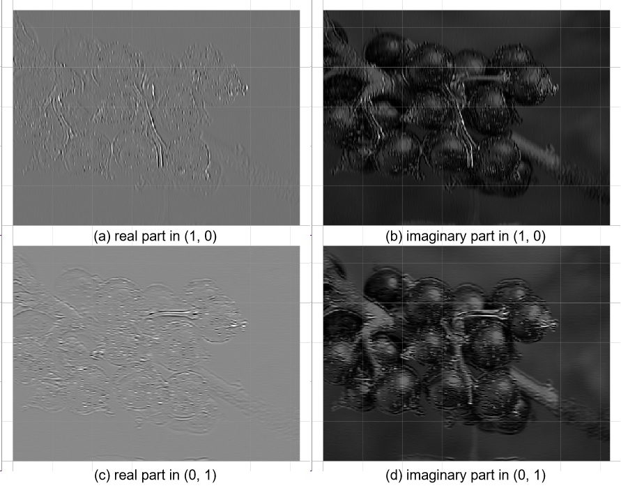
Figure 4.20 gabor filtering applied on image processing

Note

Gabor kernel is defined as a gaussian envelope, multiplied with a sine harmonic function. However, when dealing with data in different dimensions, its form might be different since in different coordinate systems (e.g. cartesian or polar in dimension 2, or spherical frame in dimension 3).

For most libraries, they has presumed the dimensions of data to be processed therefore it is difficult to use a consistent method to obtain the Gabor kernel. Based on definition, the multivariate gaussian is handy to be obtained, so the keypoint is the generalization for sine function into n-dimension.

Consider the degeneracy of degree fo freedom (DoF) occurs (see topic degeneracy), for sine function, in 1D line (DoF=1), value varies in each point (DoF=0); in 2D plane (DoF=2), value varies in each line (DoF=1); for 3D volume (DoF=3), value varies in each plane (DoF=2). Generally, for n-dimension case, if a 1-dimension degenerated hyperplane is defined, the sine function will be described as simple as that in 1-dimension. Here, we use normal to define those hyperplanes, through which the spatial sine function can be implemented in different dimensions with the identical interface:

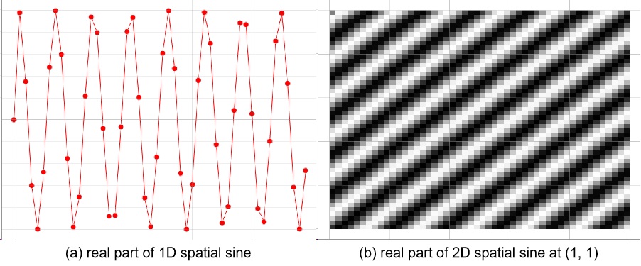
Figure 4.21 real part of spatial sine in different dimensions

Then multiply them into the corresponding multivariate gaussian, the gabor kernel will be obtained as:

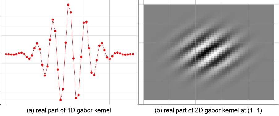
Figure 4.22 real part of gabor kernel in different dimensions

4.3.1.3. Curvature of image

The study of image curvature presents a fundamental understanding of the shape and deformation of objects within a digital image. Curvature, a measure of the rate of change in direction of a curve at a given point, is a critical geometric property in computer vision and image processing. In this context, curvature analysis refers to the quantitative evaluation of the deviation from straightness in the contours or boundaries of objects in an image (as shown in Figure 4.23).

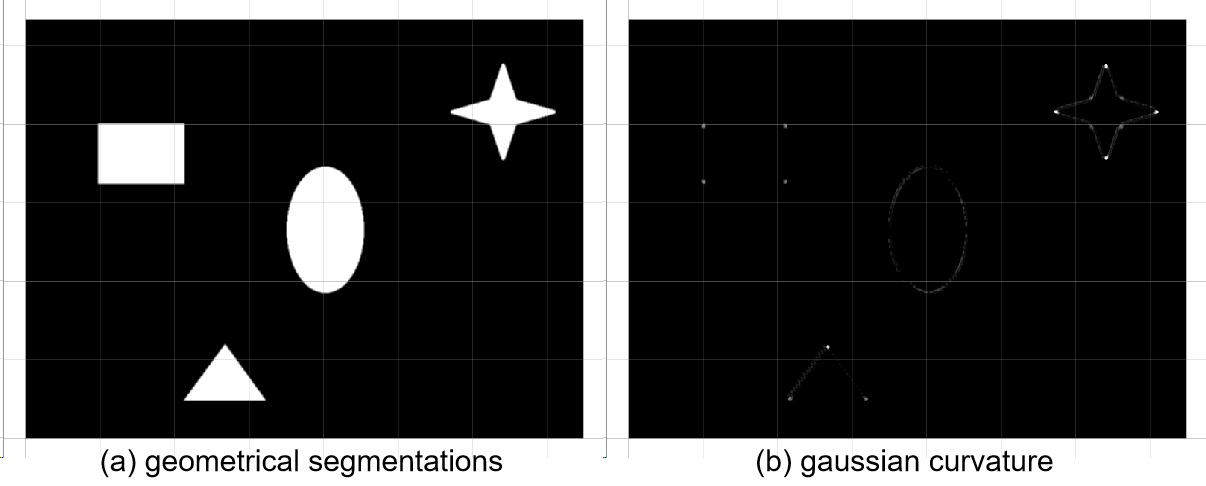
Figure 4.23 effect of gaussian curvature via hessian filter

Text here…

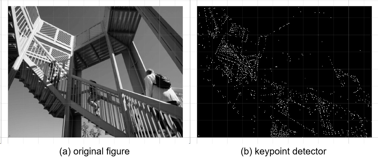
Figure 4.24 keypoint determination through curvature

---

Authors:

Chen Zhang

Version:

0.0.5

Created on:

Jun 28, 2023