4.2.6. Bayesian statistics

Bayesian statistics represents a powerful paradigm that offers a probabilistic framework for updating beliefs and making inferences in the face of uncertainty. Rooted in the foundational works of Thomas Bayes and later refined by prominent statisticians, it incorporates prior knowledge or beliefs, along with observed data, to form posterior distributions, thereby enabling more informed decision-making.

This methodology finds extensive applications across diverse domains, where dealing with incomplete or uncertain information is inherent. In the realm of science, Bayesian statistics has revolutionized fields such as genetics, where it aids in identifying causal variants by integrating prior biological knowledge with sequencing data. In finance, it is employed for portfolio optimization, risk assessment, and asset pricing, accounting for investors’ subjective beliefs and market dynamics.

Moreover, Bayesian approaches are indispensable in machine learning, particularly for tasks involving classification, regression, and clustering, where they facilitate the integration of prior assumptions into the learning process, often leading to improved model interpretability and performance. Within the field of epidemiology, Bayesian methods are employed to estimate disease prevalence, transmission rates, and the effectiveness of interventions, taking into account the inherent uncertainties surrounding disease spread.

The language of Bayesian statistics is formal and rigorous, relying on mathematical notation to describe probability distributions and update rules. Its appeal lies in its ability to provide a coherent and principled framework for integrating diverse sources of information, making it an invaluable tool for researchers and practitioners alike who seek to navigate the complexities of decision-making under uncertainty.

4.2.6.1. The basic theories

In terms of classical statistics, the statistical model of probability customarily utilize the maximum likelihood estimation (MLE) to solve the interested distribution. For an observed data set \(\mathcal{D}\), assume there is a statistical model and its corresponding parameter \(\theta\). The MLE approach actually calculate the \(\arg\max_{\theta} p(\mathcal{D} | \theta)\). In this manner, parameter \(\theta\) is nothing else but a numerical solution.

While in the Bayesian context, if it identically assumes a statistical model with parameter \(\theta\), as well as an observed data \(\mathcal{D}\), according to the Bayesian theorem:

(4.54)\[p(\theta | \mathcal{D}) = \frac{p(\mathcal{D} | \theta) p(\theta)}{p(\mathcal{D})}\]

In this circumstance, parameter \(\theta\) is a sort of probabilistic distribution instead. In the Equation 4.54, the term \(p(\mathcal{D} | \theta)\) is precisely the likelihood function in MLE approach. The distribution \(p(\theta)\) is called the Bayesian prior while the \(p(\theta | \mathcal{D})\) is termed as Bayesian posterior.

For convenience, the denominator of Equation 4.54 is a parameter \(\theta\) independent distribution that is reducible as a certain constant during calculation. Therefore it generally employs \(p(\theta | \mathcal{D}) \propto p(\mathcal{D} | \theta) p(\theta)\) for further calculations. And also, during reduction it concerns more about the parameter related term. If a kernel like term unveiled during simplification, the corresponding distribution can be established rationally.

Generally, the \(p(\theta)\) and \(p(\theta | \mathcal{D})\) are of the identical family of probabilistic distribution, therefore the Bayesian prior and posterior are relative concepts. A updated Bayesian model with calculated posterior, can be treated as prior for following learning tasks as well, through which manner the Bayesian model can possess the property of self adaption to variation data.

Another important concept in Bayesian context, is that the prediction is also probabilistic distribution instead of concrete numerics. As illustrated in the Figure 4.11, the observed data \(\mathcal{D}\) and the variable \(x^*\) are both in dependence with the parameter \(\theta\).

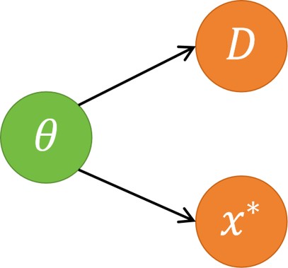
Figure 4.11 graphical model of Bayesian predictive distribution

Based on the graphical model in Figure 4.11, the joint probability of \(\theta\), \(x^*\) and \(\mathcal{D}\) is \(p(\theta, x^*, \mathcal{D}) = p(x^* | \theta) p(\mathcal{D} | \theta) p(\theta)\). Consider the Equation 4.54, the posterior joint probability \(p(x^*, \theta | \mathcal{D})\) will be:

(4.55)\[\begin{split}p(x^*, \theta | \mathcal{D}) &= \frac{p(x^* | \theta) p(\mathcal{D} | \theta) p(\theta)}{p(\mathcal{D})} \\ &= p(x^* | \theta) p(\theta | \mathcal{D})\end{split}\]

For prediction, it can be formulated via the marginalization on the parameter \(\theta\) through \(p(x^*) = \int p(x^* | \theta) p(\theta) d\theta\). As the conjugate property of \(p(\theta)\) and \(p(\theta | \mathcal{D})\), if it substitutes the \(p(\theta)\) by \(p(\theta | \mathcal{D})\), the Bayesian posterior predictive distribution can be obtained:

(4.56)\[p(x^*) = \int p(x^*, \theta | \mathcal{D}) d\theta = \int p(x^* | \theta) p(\theta | \mathcal{D}) d\theta\]

4.2.6.2. Discrete distribution family

For a comprehensive understanding on the relationship among majority of common discrete distributions, Table 4.3 lists the typical sort of distributions in accordance with the trial times \(n\), as well as the number of categories \(K\).

Table 4.3 relationship of discrete distributions

trials \(n\), categories \(K\)	\(K = 2\)	\(K > 2\)
\(n = 1\)	bernoulli	categorical
\(n > 1\)	binomial	multinomial

For general, the format of multinomial distribution with \(n\) trials and \(K\) can be preferentially investigated, due to it actually the super set of the three other ones. When \(K = 2\), it collapses to categorical distribution; when \(n = 1\), it collapses to the binomial one. While for simultaneously \(K = 2\) and \(n = 1\), the bernoulli distribution.

In addition, such mathematical degeneration similarly exists in their conjugate prior distributions. For categorical or multinomial distributions, the dirichlet distribution is always considered as the prior. When the number of categories is 2, it uses beta distribution instead. However, beta distribution is merely a specific kind of dirichlet distribution with only 2 parameters.

4.2.6.2.1. Multinomial distribution

Without loss of generality, following interpretation and deduction will be conducted within the context of multinomial distribution.

(4.57)\[\begin{split}p(\boldsymbol{\pi} | \boldsymbol{m}, M) &\propto p(\boldsymbol{m} | \boldsymbol{\pi}, M) p(\boldsymbol{\pi}) \\ &= \{ \prod_{n=1}^{N} \mathrm{Mult}(\boldsymbol{m}_n | \boldsymbol{\pi}) \} \mathrm{Dir}(\boldsymbol{\pi} | \boldsymbol{\alpha})\end{split}\]

Convert the calculation to logarithm space, and combine the \(\boldsymbol{\pi}\) independent factors into constant, the Equation 4.57 can be further simplified as:

(4.58)\[\begin{split}\ln p(\boldsymbol{\pi} | \boldsymbol{m}, M) &= \sum_{n=1}^N \ln \mathrm{Mult}(\boldsymbol{m}_n | \boldsymbol{\pi}, M) + \ln \mathrm{Dir}(\boldsymbol{\pi} | \boldsymbol{\alpha}) + C_1 \\ &= \sum_{n=1}^N \sum_{k=1}^{K} {m}_{n, k} \ln \pi_k + \sum_{k=1}^K (\alpha_k - 1) \ln \pi_k + C_2 \\ &= \sum_{k=1}^K (\sum_{n=1}^N {m}_{n, k} + \alpha_k - 1) \cdot \ln \pi_k + C_3\end{split}\]

Due to \(p(\boldsymbol{\pi} | \boldsymbol{m}, M)\) is a probability distribution, an extra term that can counteract the effect of \(C_3\) then satisfy the normalization condition should be added unconstrainedly when convert the Equation 4.58 into standard format. Here is unnecessary to make further discussion. The final expression of Equation 4.58 showed that the Bayesian posterior of \(p(\boldsymbol{\pi} | \boldsymbol{m}, M)\) is exactly the kernel of a dirichlet distribution \(\mathrm{Dir}(\boldsymbol{\pi} | \hat{\boldsymbol{\alpha}})\), with \(\hat{\boldsymbol{\alpha}}\) which satisfies:

(4.59)\[\hat{\alpha}_k = \sum_{n=1}^N {m}_{n, k} + \alpha_k\]

As for the posterior predictive distribution of multinomial, apply the Equation 4.56, the \(\boldsymbol{\pi}\) marginalized distribution will be like:

(4.60)\[\begin{split}p(\boldsymbol{m}^* | M) &= \int p(\boldsymbol{m}^* | \boldsymbol{\pi}, M) p(\boldsymbol{\pi}) d\boldsymbol{\pi} \\ &= \int \mathrm{Mult}(\boldsymbol{m}^* | \boldsymbol{\pi}, M) \mathrm{Dir}(\boldsymbol{\pi}|\boldsymbol{\alpha}) d\boldsymbol{\pi} \\ &= \int M! \prod_{k=1}^K \frac{\pi_k^{m^*_k}}{m^*_k !} \frac{\Gamma(\sum_{k=1}^K \alpha_k)}{\prod_{k=1}^K \Gamma(\alpha_k)} \prod_{k=1}^K \pi_k^{\alpha_k - 1} d\boldsymbol{\pi} \\ &= \frac{M!}{\prod_{k=1}^K m^*_k !} \cdot \frac{\Gamma(\sum_{k=1}^K \alpha_k)}{\prod_{k=1}^K \Gamma(\alpha_k)} \int \prod_{k=1}^K \pi_k^{m^*_k + \alpha_k - 1} d\boldsymbol{\pi} \\ &= \frac{M!}{\prod_{k=1}^K m^*_k !} \cdot \frac{\Gamma(\sum_{k=1}^K \alpha_k) \prod_{k=1}^K \Gamma(m^*_k + \alpha_k)}{\prod_{k=1}^K \Gamma(\alpha_k) \Gamma(\sum_{k=1}^K (m^*_k + \alpha_k))} \cdot \int \frac{\Gamma(\sum_{k=1}^K (m^*_k + \alpha_k))}{\prod_{k=1}^K \Gamma(m^*_k + \alpha_k)} \prod_{k=1}^K \pi_k^{m^*_k + \alpha_k - 1} d\boldsymbol{\pi} \\ &= \frac{M!}{\prod_{k=1}^K m^*_k !} \cdot \frac{\Gamma(\sum_{k=1}^K \alpha_k) \prod_{k=1}^K \Gamma(m^*_k + \alpha_k)}{\prod_{k=1}^K \Gamma(\alpha_k) \Gamma(\sum_{k=1}^K (m^*_k + \alpha_k))} \cdot \int \mathrm{Dir} (\boldsymbol{\pi} | \boldsymbol{\alpha} + \boldsymbol{m}^*) d\boldsymbol{\pi} \\ &\propto \prod_{k=1}^K \frac{\Gamma(m^*_k + \alpha_k)}{m^*_k ! \cdot \Gamma(\alpha_k)}\end{split}\]

The last step can be established because \(\sum_{k=1}^K m^*_k = M\). From Equation 4.60 it can finally deduce that it is the kernel of a dirichlet-multinomial distribution with parameter \(M\) and \(\boldsymbol{\alpha}\) (see [Glüsenkamp]). Consider the conjugate property of dirichlet prior as for multinomial distribution, replace the \(\mathrm{Dir}(\boldsymbol{\pi} | \boldsymbol{\alpha})\) by \(\mathrm{Dir}(\boldsymbol{\pi} | \hat{\boldsymbol{\alpha}})\) then the Bayesian posterior of multinomial can be obtained.

Here it have to consider two sorts of special cases. The first one is \(M = 1\). Under that constraint, the main likelihood function will become categorical distribution according to Table 4.3. Its Bayesian posterior still keep the form of Equation 4.58 but all of the variables (\(m_{n, k}\) and \(m^*_k\)) take the domain of \(\{0, 1\}\) instead of \(\{0, 1, \dots, M\}\). The posterior of categorical distribution is consequently still dirichlet distribution with parameter in accordance with Equation 4.59 as well. However for its posteriori predictive, consider the \(0! = 1! = 1\), the \(p(\boldsymbol{m}^*)\) is actually:

(4.61)\[p (\boldsymbol{m}^*) = \frac{\Gamma(\sum_{k=1}^K \alpha_k) \prod_{k=1}^K \Gamma(m^*_k + \alpha_k)}{\prod_{k=1}^K \Gamma(\alpha_k) \Gamma(\sum_{k=1}^K (m^*_k + \alpha_k))}\]

Consider the probability of \(p(m^*_{k^\prime} = 1)\), because the \(\sum_{k=1}^K m^*_k = 1\) and the property \(\Gamma(x + 1) = x \Gamma(x)\) of gamma function, the Equation 4.61 can be further simplified as:

(4.62)\[\begin{split}p (m^*_{k^\prime} = 1) &= \frac{\Gamma(\sum_{k=1}^K \alpha_k) \Gamma(1 + \alpha_{k^\prime}) \prod_{k^c \neq k^\prime} \Gamma(\alpha_{k^c})}{\prod_{k=1}^K \Gamma(\alpha_k) \Gamma(\sum_{k=1}^K \alpha_k + 1)} \\ &= \frac{\Gamma(\sum_{k=1}^K \alpha_k) \cdot \alpha_{k^\prime} \cdot \Gamma(\alpha^{k^\prime})}{(\sum_{k=1}^K \alpha_k) \cdot \Gamma(\sum_{k=1}^K \alpha_k) \cdot \Gamma(\alpha_{k^\prime})} \\ & = \frac{\alpha_{k^\prime}}{\sum_{k=1}^K \alpha_k}\end{split}\]

Therefore the Bayesian posterior predictive of categorical distribution is another categorical one noted as \(\mathrm{Cat}(\boldsymbol{m}^* | \{\frac{\alpha_k}{\sum_{i=1}^K \alpha_i}\}_{k=1}^K)\).

The second special case is for the binomial distribution with constraint \(K = 2\). In that condition, the Equation 4.58 has only two parameters \(\alpha_1\) and \(\alpha_2\), the dirichlet prior will collapse to the beta distribution \(\mathrm{Beta}(x | \alpha_1, \alpha_2)\) as well. Its predictive also convert correspondingly like:

(4.63)\[\begin{split}p (m^*_1 | M) &\propto \frac{\Gamma(m^*_1 + \alpha_1)}{m^*_1 ! \Gamma(\alpha_1)} \cdot \frac{\Gamma(M - m^*_1 + \alpha_2)}{(M - m^*_1)! \Gamma(\alpha_2)} \\ &\propto \frac{M!}{m^*_1 ! (M - m^*_1) !} \cdot \frac{\Gamma(m^*_1 + \alpha_1) \Gamma(M - m^*_1 + \alpha_2)}{ \Gamma(M + \alpha_1 + \alpha_2)} \cdot \frac{\Gamma(\alpha_1 + \alpha_2)}{\Gamma(\alpha_1) \Gamma(\alpha_2)}\end{split}\]

Which is exactly the kernel of a certain beta binomial distribution.

If simultaneously consider the \(M = 1\) and \(K = 2\). It can be conducted for the bernoulli likelihood, its Bayesian posterior is beta distribution, while its predictive is another bernoulli.

For conclusion, the common likelihood functions with discrete distribution family can be summarized in the Table 4.4:

Table 4.4 Bayesian statistics of discrete distributions

likelihood	parameter	condition	conjugate	predictive
bernoulli	\(p\)	\(-\)	beta	bernoulli
binomial	\(p\)	\(M\)	beta	beta binomial
categorical	\(\boldsymbol{\pi}\)	\(-\)	dirichlet	categorical
multinomial	\(\boldsymbol{\pi}\)	\(M\)	dirichlet	dirichlet multinomial

4.2.6.2.2. Poisson distribution

Poisson distribution is a discrete probability distribution that models the probability of a given number of events occurring in a fixed interval of time or space, given that these events occur with a known average rate and independently of each other. It is commonly used in various fields such as statistics, probability theory, and even in some applications of artificial intelligence.

As for the poisson likelihood function, its conjugate prior and posterior are of gamma distributions. Let \(p(x | \lambda) = \mathrm{Poi}(x | \lambda)\), \(p(x) = \mathrm{Gam}(\lambda | a, b)\), and \(N\) non-negative observations \(\textbf{X} = \{x_1, \dots, x_N \}\), its Bayesian posterior will be like:

(4.64)\[\begin{split}p(\lambda | \textbf{X}) &\propto p(\textbf{X} | \lambda) p(\lambda) \\ &= \{ \prod_{n=1}^N \mathrm{Poi}(x_n | \lambda) \} \mathrm{Gam}(\lambda | a, b)\end{split}\]

For convenience, conduct the reduction in logarithmic space:

(4.65)\[\begin{split}\ln p(\lambda | \textbf{X}) &= \sum_{n=1}^N \ln \mathrm{Poi}(x_n | \lambda) + \ln \mathrm{Gam}(\lambda | a, b) + C_1 \\ &= \sum_{n=1}^N \{ x_n \ln \lambda - \ln x_n ! - \lambda \} + (a-1) \ln \lambda - b \ln \lambda + \ln \left( \frac{b^a}{\Gamma(a)} \right) + C_1 \\ &= (\sum_{n=1}^N x_n + a - 1) \ln \lambda - (N + b) \lambda + C_2\end{split}\]

The final step of Equation 4.65 is established because that for \(p(\lambda | \textbf{X})\), the variable \(\lambda\) involved terms are just \(\lambda\) and \(\ln \lambda\). Other \(\lambda\) independent factors are all included into the constant \(C_2\). The posterior of Equation 4.65 obviously reveals the kernel of a gamma \(\mathrm{Gam}(\lambda | \hat{a}, \hat{b})\), with parameters \(\hat{a}\) and \(\hat{b}\) that satisfies:

(4.66)\[\begin{split}\hat{a} &= \sum_{n=1}^N x_n + a \\ \hat{b} &= N + b\end{split}\]

And for the predictive:

(4.67)\[\begin{split}p(x^*) &= \int p(x^* | \lambda) p(\lambda) d\lambda \\ &= \int \frac{\lambda^{x^*}}{x^* !} e^{-\lambda} \frac{b^a}{\Gamma(a)} \lambda^{a-1} e^{-b\lambda} d\lambda \\ &= \frac{b^a}{x^* ! \Gamma(a)} \cdot \frac{\Gamma(x^* + a)}{(x^* + a)^{(1 + b)}} \int \frac{(x^* + a)^{(1 + b)} }{\Gamma(x^* + a)} \lambda^{x^* + a - 1} e^{-(1+b)\lambda} d\lambda \\ &= \frac{b^a}{x^* ! \Gamma(a)} \cdot \frac{\Gamma(x^* + a)}{(x^* + a)^{(1 + b)}} \int \mathrm{Gam}(\lambda | x^* + a, 1 + b) d\lambda \\ &= \frac{b^a}{x^* ! \Gamma(a)} \cdot \frac{\Gamma(x^* + a)}{(x^* + a)^{(1 + b)}} \\ &= \frac{\Gamma(x^* + a)}{x^* ! \Gamma(a)} \cdot (\frac{1}{b+1})^{x^*} (1-\frac{1}{b+1})^a\end{split}\]

Thus, the predictive of poisson distribution is a negative binomial distribution with parameter \(a\) and \((1+b)^{-1}\). As for its Bayesian posterior predictive, replace the \(a\) and \(b\) by \(\hat{a}\) and \(\hat{b}\) as showed in Equation 4.66.

4.2.6.3. Continuous distribution family

Gauss, also called normal distribution, is a conventional but widely used continuous distribution. In statistics and probability theory, beyond its fundamental role in describing natural phenomena and modeling error distributions, the normal distribution has evolved to serve as a cornerstone in statistical inference. In hypothesis testing, for instance, the null hypothesis is often assumed to follow a normal distribution under certain conditions, allowing researchers to determine the statistical significance of their findings. This framework has facilitated groundbreaking discoveries in numerous scientific disciplines, where the precision and reliability of conclusions are paramount.

As for Gauss likelihood function, it is acceptable for 3 different types of conjugate priors. Similarly without loss of generality, all following reduction will be conducted in the context of multivariate Gauss. The properties of univariate one will be further investigated through distribution degeneration. For convenience, here introduces precision matrix \(\boldsymbol{\Lambda}\) which is the inverse of covariance matrix \(\boldsymbol{\Sigma}\) of Gauss (\(\mathcal{N}(\boldsymbol{x}|\boldsymbol{\mu}, \boldsymbol{\Sigma})\) is equivalent to \(\mathcal{N}(\boldsymbol{x}|\boldsymbol{\mu}, \boldsymbol{\Lambda}^{-1})\)).

• Gauss prior

For the likelihood \(\mathcal{N}(\boldsymbol{x} | \boldsymbol{\mu}, \boldsymbol{\Lambda}^{-1})\), the prior of another Gauss \(\mathcal{N}(\boldsymbol{\mu} | \boldsymbol{m}, \boldsymbol{\Lambda}_{\boldsymbol{\mu}}^{-1})\) is the framework to infer the unknown mean \(\boldsymbol{\mu}\). In that case, the precision \(\boldsymbol{\Lambda}\) is the given condition during whole calculation.

Therefore for \(N\) observations \(\boldsymbol{X} = \{\boldsymbol{x}_1, \dots, \boldsymbol{x}_N\}\), its Bayesian posterior will be:

(4.68)\[\begin{split}p(\boldsymbol{\mu} | \boldsymbol{X}) &\propto p(\boldsymbol{X} | \boldsymbol{\mu}) p(\boldsymbol{\mu}) \\ &= \left\{ \prod_{n=1}^N \mathcal{N}(\boldsymbol{x}_n | \boldsymbol{\mu}, \boldsymbol{\Lambda}^{-1}) \right\} \mathcal{N}(\boldsymbol{\mu} | \boldsymbol{m}, \boldsymbol{\Lambda}_{\boldsymbol{\mu}}^{-1})\end{split}\]

Conduct further calculation in logarithmic space:

(4.69)\[\begin{split}\ln p(\boldsymbol{\mu} | \boldsymbol{X}) &= \sum_{n=1}^N \ln \mathcal{N}(\boldsymbol{x}_n | \boldsymbol{\mu}, \boldsymbol{\Lambda}^{-1}) + \ln \mathcal{N}(\boldsymbol{\mu} | \boldsymbol{m}, \boldsymbol{\Lambda}_{\boldsymbol{\mu}}^{-1}) + C_1 \\ &= -\frac{1}{2} \left\{ \sum_{n=1}^N (\boldsymbol{x}_n - \boldsymbol{\mu})^\top \boldsymbol{\Lambda} (\boldsymbol{x}_n - \boldsymbol{\mu}) + (\boldsymbol{\mu} - \boldsymbol{m})^\top \boldsymbol{\Lambda}_{\boldsymbol{\mu}} (\boldsymbol{\mu} - \boldsymbol{m}) \right\} + C_2 \\ &= -\frac{1}{2} \left\{ \boldsymbol{\mu}^\top (N\boldsymbol{\Lambda} + \boldsymbol{\Lambda}_{\boldsymbol{\mu}}) \boldsymbol{\mu} - 2\boldsymbol{\mu}^\top (\boldsymbol{\Lambda} \sum_{n=1}^N \boldsymbol{x}_n + \boldsymbol{\Lambda}_{\boldsymbol{\mu}} \boldsymbol{m}) \right\} + C_3 \\ &= -\frac{1}{2} \left\{ \boldsymbol{\mu}^\top \hat{\boldsymbol{\Lambda}}_{\boldsymbol{\mu}} \boldsymbol{\mu} - 2 \boldsymbol{\mu}^\top \hat{\boldsymbol{\Lambda}}_{\boldsymbol{\mu}} \hat{\boldsymbol{m}} \right\} + C_3 \\ &= -\frac{1}{2} \left\{ (\boldsymbol{\mu}-\hat{\boldsymbol{m}})^\top \hat{\boldsymbol{\Lambda}}_{\boldsymbol{\mu}} (\boldsymbol{\mu} - \hat{\boldsymbol{m}}) \right\} + C_4\end{split}\]

Thus, the Bayesian posterior of Gauss used Gauss prior is also another Gauss distribution \(\mathcal{N}(\boldsymbol{\mu} | \hat{\boldsymbol{m}}, \hat{\boldsymbol{\Lambda}}_{\boldsymbol{\mu}}^{-1})\) with parameters of \(\hat{\boldsymbol{m}}\) and \(\hat{\boldsymbol{\Lambda}}_{\boldsymbol{\mu}}\) where:

(4.70)\[\begin{split}\hat{\boldsymbol{\Lambda}}_{\boldsymbol{\mu}} &= N\boldsymbol{\Lambda} + \boldsymbol{\Lambda}_{\boldsymbol{\mu}} \\ \hat{\boldsymbol{m}} &= \hat{\boldsymbol{\Lambda}}_{\boldsymbol{\mu}}^{-1} (\boldsymbol{\Lambda} \sum_{n=1}^N \boldsymbol{x}_n + \boldsymbol{\Lambda}_{\boldsymbol{\mu}} \boldsymbol{m})\end{split}\]

Because \(p(\boldsymbol{x}^*|\boldsymbol{\mu}) \propto p(\boldsymbol{\mu}|\boldsymbol{x}^*) p(\boldsymbol{x}^*)\), the predictive under Gauss prior can be calculated via:

(4.71)\[\ln p(\boldsymbol{x}^*) = \ln p(\boldsymbol{x}^* | \boldsymbol{\mu}) - \ln p(\boldsymbol{\mu}|\boldsymbol{x}^*) + C\]

Where the \(p(\boldsymbol{\mu}|\boldsymbol{x}^*)\) can be defined as taking one \(\boldsymbol{x}^*\) sample. Thus, from Equation 4.70, the \(p(\boldsymbol{x}^*|\boldsymbol{\mu})\) will be:

(4.72)\[\begin{split}p(\boldsymbol{x}^*|\boldsymbol{\mu}) &= \mathcal{N} (\boldsymbol{\mu} | (\boldsymbol{\Lambda} + \boldsymbol{\Lambda}_\boldsymbol{\mu})^{-1} (\boldsymbol{\Lambda x}^* + \boldsymbol{\Lambda_{\mu} m}), (\boldsymbol{\Lambda} + \boldsymbol{\Lambda}_\boldsymbol{\mu})^{-1}) \\ &= \mathcal{N} (\boldsymbol{\mu} | \boldsymbol{m}(\boldsymbol{x}^*), (\boldsymbol{\Lambda} + \boldsymbol{\Lambda}_\boldsymbol{\mu})^{-1})\end{split}\]

In this circumstance, consider the \(\boldsymbol{\Lambda}\) and \(\boldsymbol{\Lambda_{\mu}}\) are both symmetric matrices, the Equation 4.71 can be simplified by the following steps:

(4.73)\[\begin{split}\ln p(\boldsymbol{x}^*) =& -\frac{1}{2} (\boldsymbol{x}^* - \boldsymbol{\mu})^\top \boldsymbol{\Lambda} (\boldsymbol{x}^* - \boldsymbol{\mu}) + \frac{1}{2} \left\{ \left[\boldsymbol{\mu} -\boldsymbol{m}(\boldsymbol{x}^*) \right]^\top (\boldsymbol{\Lambda} + \boldsymbol{\Lambda}_\boldsymbol{\mu}) \left[ \boldsymbol{\mu} - \boldsymbol{m}(\boldsymbol{x}^*) \right] \right\} + C_1 \\ \propto& -\frac{1}{2} \left[ \boldsymbol{x}^{*\top} \boldsymbol{\Lambda} \boldsymbol{x}^* - 2 \boldsymbol{x}^{*\top} \boldsymbol{\Lambda} \boldsymbol{\mu} + C_2 \right] + \frac{1}{2} \left[ \boldsymbol{m}(\boldsymbol{x}^*)^\top (\boldsymbol{\Lambda} + \boldsymbol{\Lambda}_\boldsymbol{\mu}) \boldsymbol{m}(\boldsymbol{x}^*) - 2 \boldsymbol{\mu}^\top (\boldsymbol{\Lambda} + \boldsymbol{\Lambda}_\boldsymbol{\mu}) \boldsymbol{m}(\boldsymbol{x}^*) + C_3 \right] \\ \propto& -\frac{1}{2} \left[ \boldsymbol{x}^{*\top} \boldsymbol{\Lambda} \boldsymbol{x}^* - 2 \boldsymbol{x}^{*\top} \boldsymbol{\Lambda} \boldsymbol{\mu} \right] + \frac{1}{2} \left\{ (\boldsymbol{\Lambda x}^* + \boldsymbol{\Lambda_{\mu} m})^\top \left[ (\boldsymbol{\Lambda} + \boldsymbol{\Lambda}_\boldsymbol{\mu})^{-1} \right]^\top (\boldsymbol{\Lambda} + \boldsymbol{\Lambda}_\boldsymbol{\mu}) (\boldsymbol{\Lambda} + \boldsymbol{\Lambda}_\boldsymbol{\mu})^{-1} (\boldsymbol{\Lambda x}^* + \boldsymbol{\Lambda_{\mu} m}) \right\} \\ &- \left[ \boldsymbol{\mu}^\top (\boldsymbol{\Lambda} + \boldsymbol{\Lambda}_\boldsymbol{\mu}) (\boldsymbol{\Lambda} + \boldsymbol{\Lambda}_\boldsymbol{\mu})^{-1} (\boldsymbol{\Lambda x}^* + \boldsymbol{\Lambda_{\mu} m}) + C_3 \right] \\ =& -\frac{1}{2} \left[ \boldsymbol{x}^{*\top} \boldsymbol{\Lambda} \boldsymbol{x}^* - 2 \boldsymbol{x}^{*\top} \boldsymbol{\Lambda} \boldsymbol{\mu} \right] + \frac{1}{2} \left[ \boldsymbol{x}^* \boldsymbol{\Lambda} (\boldsymbol{\Lambda} + \boldsymbol{\Lambda}_\boldsymbol{\mu})^{-1} \boldsymbol{\Lambda x}^* + 2 \boldsymbol{x}^{*\top} \boldsymbol{\Lambda} (\boldsymbol{\Lambda} + \boldsymbol{\Lambda}_\boldsymbol{\mu})^{-1} \boldsymbol{\Lambda_{\mu} m} - 2 \boldsymbol{x}^{*\top} \boldsymbol{\Lambda \mu} + C_4 \right] \\ =& -\frac{1}{2} \left\{ \boldsymbol{x}^{*\top} \left[ \boldsymbol{\Lambda} - \boldsymbol{\Lambda} (\boldsymbol{\Lambda} + \boldsymbol{\Lambda_\mu})^{-1} \boldsymbol{\Lambda} \right] \boldsymbol{x}^* - 2 \boldsymbol{x}^{*\top} \boldsymbol{\Lambda} (\boldsymbol{\Lambda} + \boldsymbol{\Lambda_\mu})^{-1} \boldsymbol{\Lambda_\mu m} \right\} + C_5\end{split}\]

Therefore, its Bayesian predictive is still a sort of Gauss distribution \(\mathcal{N}(\boldsymbol{x}^* | \boldsymbol{\mu}^*, \boldsymbol{\Lambda}^{* -1})\) that:

(4.74)\[\begin{split}\boldsymbol{\Lambda}^* &= \boldsymbol{\Lambda} - \boldsymbol{\Lambda} (\boldsymbol{\Lambda} + \boldsymbol{\Lambda_\mu})^{-1} \boldsymbol{\Lambda} \\ &= \boldsymbol{\Lambda} - \boldsymbol{\Lambda I} (\boldsymbol{\Lambda} + \boldsymbol{\Lambda_\mu})^{-1} \boldsymbol{I \Lambda} \\ &= (\boldsymbol{\Lambda}^{-1} + \boldsymbol{I \Lambda_{\mu}}^{-1} \boldsymbol{I})^{-1} \\ &= (\boldsymbol{\Lambda}^{-1} + \boldsymbol{\Lambda_{\mu}}^{-1})^{-1} \\ \boldsymbol{\mu}^* &= \boldsymbol{\Lambda}^{* -1} \boldsymbol{\Lambda} (\boldsymbol{\Lambda} + \boldsymbol{\Lambda_\mu})^{-1} \boldsymbol{\Lambda_\mu m} \\ &= \boldsymbol{\Lambda}^{* -1} \boldsymbol{\Lambda} [\boldsymbol{\Lambda}^{-1} - \boldsymbol{\Lambda}^{-1} \boldsymbol{\Lambda}^* \boldsymbol{\Lambda}^{-1}] \boldsymbol{\Lambda_{\mu} m} \\ &= (\boldsymbol{\Lambda}^{* -1} \boldsymbol{\Lambda_{\mu}} - \boldsymbol{\Lambda}^{-1} \boldsymbol{\Lambda_{\mu}}) \boldsymbol{m} \\ & = (\boldsymbol{\Lambda}^{-1} + \boldsymbol{\Lambda_{\mu}}^{-1} - \boldsymbol{\Lambda}^{-1}) \boldsymbol{\Lambda_{\mu} m} = \boldsymbol{m}\end{split}\]

The reduction of Equation 4.74 can be established by Sherman–Morrison–Woodbury formula (see [Higham2002]). As for Bayesian posterior predictive, replace all the \(\boldsymbol{m}\) and \(\boldsymbol{\Lambda_{\mu}}\) by \(\hat{\boldsymbol{m}}\) and \(\hat{\boldsymbol{\Lambda}}_{\boldsymbol{\mu}}\) as noted in Equation 4.70.

If it confines all \(\boldsymbol{\mu}\) related variables \(\in \mathbb{R}^1\), and all \(\boldsymbol{\Lambda}\) ones are \(\in \mathbb{R}^{1 \times 1}\) (e.g. \(\lambda = \sigma^2\)), all above conclusions can be applied in univariate Gauss.

• Wishart prior

For the likelihood \(\mathcal{N}(\boldsymbol{x} | \boldsymbol{\mu}, \boldsymbol{\Lambda}^{-1})\), the prior of a Wishart distribution \(\mathcal{W}(\boldsymbol{\Lambda} | \mu, \boldsymbol{W})\) is the framework to infer the unknown precision \(\boldsymbol{\Lambda}\). Conditions of \(\boldsymbol{W} \in \mathbb{R}^{D \times D}\) and \(\nu > D - 1\) are established. In that case, the mean vector \(\boldsymbol{\mu}\) is the given condition during whole calculation.

Therefore for \(N\) observations \(\boldsymbol{X} = \{\boldsymbol{x}_1, \dots, \boldsymbol{x}_N\}\), its Bayesian posterior will be:

(4.75)\[\begin{split}\ln p(\boldsymbol{\Lambda} | \boldsymbol{X}) &\propto \ln \left\{ \left[ \prod_{n=1}^N \mathcal{N}(\boldsymbol{x}_n | \boldsymbol{\mu}, \boldsymbol{\Lambda}^{-1}) \right] \mathcal{W}(\boldsymbol{\Lambda} | \nu, \boldsymbol{W}) \right\} + C_1 \\ &= \sum_{n=1}^N \ln \mathcal{N} (\boldsymbol{x}_n | \boldsymbol{\mu}, \boldsymbol{\Lambda}^{-1}) + \ln \mathcal{W} (\boldsymbol{\Lambda} | \nu, \boldsymbol{W}) + C_1 \\ &= \frac{N + \nu - D - 1}{2} \ln | \boldsymbol{\Lambda} | - \frac{1}{2} \mathrm{Tr} \left\{ [\sum_{n=1}^N (\boldsymbol{x}_n - \boldsymbol{\mu})(\boldsymbol{x}_n - \boldsymbol{\mu})^\top + \boldsymbol{W}^{-1}] \boldsymbol{\Lambda} \right\} + C_2\end{split}\]

The last step of Equation 4.75 is established because that for scalar \(\boldsymbol{x}^\top \boldsymbol{\Lambda x} = \mathrm{Tr}(\boldsymbol{x}^\top \boldsymbol{\Lambda x})\) and \(\mathrm{Tr}(\boldsymbol{ABC}) = \mathrm{Tr}(\boldsymbol{BCA}) = \mathrm{Tr}(\boldsymbol{CAB})\). Consequently, the Bayesian posterior in condition of Wishart prior is also another Wishart distribution \(\mathcal{W}(\boldsymbol{\Lambda} | \hat{\nu}, \hat{\boldsymbol{W}})\) that:

(4.76)\[\begin{split}\hat{\nu} &= N + \nu \\ \hat{\boldsymbol{W}}^{-1} &= \sum_{n=1}^N (\boldsymbol{x}_n - \boldsymbol{\mu})(\boldsymbol{x}_n - \boldsymbol{\mu})^\top + \boldsymbol{W}^{-1}\end{split}\]

Because \(p(\boldsymbol{x}^*|\boldsymbol{\Lambda})\propto p(\boldsymbol{\Lambda}|\boldsymbol{x}^*) p(\boldsymbol{x}^*)\), the predictive under Wishart prior can be calculated via:

(4.77)\[\ln p(\boldsymbol{x}^*) = \ln p(\boldsymbol{x}^* | \boldsymbol{\Lambda}) - \ln p(\boldsymbol{\Lambda} | \boldsymbol{x}^*) + C\]

Takes one \(\boldsymbol{x}^*\) sample to explicitly express the \(p(\boldsymbol{\Lambda}|\boldsymbol{x}^*)\), from the Equation 4.76, the following relationship can be ascertained:

(4.78)\[p(\boldsymbol{\Lambda} | \boldsymbol{x}^*) = \mathcal{W} (\boldsymbol{\Lambda} | 1 + \nu, [(\boldsymbol{x}^* - \boldsymbol{\mu})(\boldsymbol{x}^* - \boldsymbol{\mu})^\top + \boldsymbol{W}^{-1}]^{-1})\]

In this circumstance, the Equation 4.77 can be simplified by the following steps:

(4.79)\[\begin{split}\ln p(\boldsymbol{x}^*) =& -\frac{1}{2} (\boldsymbol{x}^* - \boldsymbol{\mu})^\top \boldsymbol{\Lambda} (\boldsymbol{x}^* - \boldsymbol{\mu}) + \frac{1}{2}\mathrm{Tr} \left\{ \left[ (\boldsymbol{x}^* - \boldsymbol{\mu})(\boldsymbol{x}^* - \boldsymbol{\mu})^\top + \boldsymbol{W}^{-1} \right]\boldsymbol{\Lambda} \right\} \\ &+ \frac{\nu+1}{2} \ln | [(\boldsymbol{x}^* - \boldsymbol{\mu})(\boldsymbol{x}^* - \boldsymbol{\mu})^\top + \boldsymbol{W}^{-1}]^{-1} | + C_1 \\ =& -\frac{\nu+1}{2} \ln | (\boldsymbol{x}^* - \boldsymbol{\mu})(\boldsymbol{x}^* - \boldsymbol{\mu})^\top + \boldsymbol{W}^{-1} | + C_2 \\ =& -\frac{\nu+1}{2} \ln | \boldsymbol{I} + \boldsymbol{W} (\boldsymbol{x}^* - \boldsymbol{\mu})(\boldsymbol{x}^* - \boldsymbol{\mu})^\top | + C_3 \\ =& -\frac{\nu+1}{2} \ln \left[1 + (\boldsymbol{x}^* - \boldsymbol{\mu})^\top \boldsymbol{W} (\boldsymbol{x}^* - \boldsymbol{\mu}) \right] + C_3\end{split}\]

The reduction process in Equation 4.79 has employed the relation \(| \boldsymbol{I} + \boldsymbol{ab}^\top | = | 1 + \boldsymbol{b}^\top \boldsymbol{a} |\). From final expression of Equation 4.79, it reveals the kernel of multivariate student-t distribution \(\mathrm{Stu}(\boldsymbol{x} | \boldsymbol{\mu}_s, \boldsymbol{\Lambda}_s, \nu_s)\) where:

(4.80)\[\begin{split}\boldsymbol{\mu}_s &= \boldsymbol{\mu} \\ \nu_s &= \nu + 1 - D \\ \boldsymbol{\Lambda}_s &= \nu_s \boldsymbol{W}\end{split}\]

For Bayesian posterior predictive in the condition of Wishart prior, replace all the \(\nu\) and \(\boldsymbol{W}\) with \(\hat{\nu}\) and \(\hat{\boldsymbol{W}}\) respectively, as noted in Equation 4.76.

If it confines all dimension related variables into the domain \(\mathbb{R}^1\), the Wishart distribution will collapse to \(\mathcal{W}(\Lambda | \nu, W)\) so that:

(4.81)\[\begin{split}\ln \mathcal{W}(\Lambda | \nu, W) &\propto \frac{\nu - 2}{2} \ln \Lambda - \frac{\Lambda}{2W} + C_1 \\ &= (\frac{\nu}{2} - 1) \ln \Lambda - \frac{1}{2W} \Lambda + C_1 \sim \ln \mathrm{Gam} (\Lambda | \frac{\nu}{2}, \frac{1}{2W})\end{split}\]

The multivariate student-t distribution will collapse to univariate one as well.

• Gauss-Wishart prior

For the likelihood \(\mathcal{N}(\boldsymbol{x} | \boldsymbol{\mu}, \boldsymbol{\Lambda}^{-1})\), if mean \(\boldsymbol{\mu}\) and precision \(\boldsymbol{\Lambda}\) are both unknown, it employs the Gaussian-Wishart distribution as conjugate prior to infer those two parameters. A Gaussian-Wishart distribution \(\mathcal{NW}(\boldsymbol{\mu}, \boldsymbol{\Lambda} | \boldsymbol{m}, \beta, \nu, \boldsymbol{W})\) can be seen as the coupling of Wishart and Gauss distribution:

(4.82)\[\begin{split}p(\boldsymbol{\mu}, \boldsymbol{\Lambda}) &= \mathcal{NW}(\boldsymbol{\mu}, \boldsymbol{\Lambda} | \boldsymbol{m}, \beta, \nu, \boldsymbol{W}) \\ &= \mathcal{N}(\boldsymbol{\mu}, \boldsymbol{\Lambda} | \boldsymbol{m}, (\beta \boldsymbol{\Lambda})^{-1}) \mathcal{W}(\boldsymbol{\Lambda} | \nu, \boldsymbol{W})\end{split}\]

In reduction, firstly uses the \(\mathcal{N}(\boldsymbol{\mu}, \boldsymbol{\Lambda} | \boldsymbol{m}, (\beta \boldsymbol{\Lambda})^{-1})\) only to infer the posterior \(\hat{\boldsymbol{m}}\) and \(\hat{\beta}\). Takes the precision \(\boldsymbol{\Lambda}\) as a given condition in this step, according to Equation 4.70, the posterior will be like:

(4.83)\[p(\boldsymbol{\mu} | \boldsymbol{\Lambda}, \boldsymbol{X}) = \mathcal{N} (\boldsymbol{\mu} | \hat{\boldsymbol{m}}, (\hat{\beta} \boldsymbol{\Lambda})^{-1})\]

Where:

(4.84)\[\begin{split}\hat{\beta} \boldsymbol{\Lambda} &= N \boldsymbol{\Lambda} + \beta \boldsymbol{\Lambda} \\ \hat{\beta} &= N + \beta \\ \hat{\boldsymbol{m}} &= (\hat{\beta} \boldsymbol{\Lambda})^{-1} (\boldsymbol{\Lambda} \sum_{n=1}^N \boldsymbol{x}_n + \beta \boldsymbol{\Lambda m}) \\ &= \frac{1}{N+\beta} (\sum_{n=1}^N \boldsymbol{x}_n + \beta \boldsymbol{m})\end{split}\]

Because the Bayesian formula:

(4.85)\[\begin{split}\because&\ p(\boldsymbol{\mu} | \boldsymbol{\Lambda}, \boldsymbol{X}) p(\boldsymbol{\Lambda} | \boldsymbol{X}) = \frac{p(\boldsymbol{X} | \boldsymbol{\mu}, \boldsymbol{\Lambda})p(\boldsymbol{\mu}, \boldsymbol{\Lambda})}{p(\boldsymbol{X})} \\ \therefore&\ \ln p(\boldsymbol{\Lambda} | \boldsymbol{X}) = \ln p(\boldsymbol{X} | \boldsymbol{\mu}, \boldsymbol{\Lambda}) + \ln p(\boldsymbol{\mu}, \boldsymbol{\Lambda}) - \ln p(\boldsymbol{\mu} | \boldsymbol{\Lambda}, \boldsymbol{X}) + C\end{split}\]

Put Equation 4.82 and Equation 4.83 into the Equation 4.85, reduce the \(\boldsymbol{\Lambda}\) related terms:

(4.86)\[\begin{split}\ln p(\boldsymbol{\Lambda} | \boldsymbol{X}) =& \ln \mathcal{N} (\boldsymbol{X} | \boldsymbol{\mu}, \boldsymbol{\Lambda}^{-1}) + \ln \mathcal{N} (\boldsymbol{\mu} | \boldsymbol{m}, (\beta \boldsymbol{\Lambda})^{-1}) + \ln \mathcal{W} (\boldsymbol{\Lambda} | \nu, \boldsymbol{W}) - \ln \mathcal{N} (\boldsymbol{\mu} | \hat{\boldsymbol{m}}, (\hat{\beta} \boldsymbol{\Lambda})^{-1}) + C_1 \\ =& \frac{1}{2} \sum_{n=1}^N [ \ln | \boldsymbol{\Lambda} | - (\boldsymbol{x}_n - \boldsymbol{\mu})^\top \boldsymbol{\Lambda} (\boldsymbol{x}_n - \boldsymbol{\mu}) ] + \frac{1}{2} [ \ln | \beta \boldsymbol{\Lambda} | - \beta (\boldsymbol{\mu} - \boldsymbol{m})^\top \boldsymbol{\Lambda} (\boldsymbol{\mu} - \boldsymbol{m}) ] \\ &+ \frac{\nu + D - 1}{2} \ln | \boldsymbol{\Lambda} | - \frac{1}{2} \mathrm{Tr}(\boldsymbol{W}^{-1} \boldsymbol{\Lambda}) - \frac{1}{2} [ \ln | \hat{\beta} \boldsymbol{\Lambda} | - \hat{\beta} (\boldsymbol{\mu} - \hat{\boldsymbol{m}})^\top \boldsymbol{\Lambda} (\boldsymbol{\mu} - \hat{\boldsymbol{m}}) ] + C_2 \\ =& \frac{1}{2} [ \hat{\beta} (\boldsymbol{\mu} - \hat{\boldsymbol{m}})^\top \boldsymbol{\Lambda} (\boldsymbol{\mu} - \hat{\boldsymbol{m}}) - \sum_{n=1}^N (\boldsymbol{x}_n - \boldsymbol{\mu})^\top \boldsymbol{\Lambda} (\boldsymbol{x}_n - \boldsymbol{\mu}) - \beta (\boldsymbol{\mu} - \boldsymbol{m})^\top \boldsymbol{\Lambda} (\boldsymbol{\mu} - \boldsymbol{m}) - \mathrm{Tr}(\boldsymbol{W}^{-1}\boldsymbol{\Lambda}) ] \\ &+ \frac{N+\nu-D-1}{2} \ln | \boldsymbol{\Lambda} | + C_3\end{split}\]

Substitute part of variables in the Equation 4.86 with Equation 4.84, the first term in Equation 4.86 will be like:

(4.87)\[\begin{split}\frac{1}{2}[\cdot] =& \frac{1}{2} [(N+\beta) \boldsymbol{\mu}^\top \boldsymbol{\Lambda \mu} - 2 \boldsymbol{\mu}^\top \boldsymbol{\Lambda} (\sum_{n=1}^N \boldsymbol{x}_n + \beta \boldsymbol{m}) + \hat{\beta} \hat{\boldsymbol{m}}^\top \boldsymbol{\Lambda} \hat{\boldsymbol{m}} - \sum_{n=1}^N \boldsymbol{x}_n^\top \boldsymbol{\Lambda} \boldsymbol{x}_n + 2\boldsymbol{\mu}^\top \boldsymbol{\Lambda} \sum_{n=1}^N \boldsymbol{x}_n \\ &- N \boldsymbol{\mu}^\top \boldsymbol{\Lambda} \boldsymbol{\mu} - \beta \boldsymbol{\mu}^\top \boldsymbol{\Lambda} \boldsymbol{\mu} + 2\beta \boldsymbol{\mu}^\top \boldsymbol{\Lambda} \boldsymbol{m} - \beta \boldsymbol{m}^\top \boldsymbol{\Lambda} \boldsymbol{m} - \mathrm{Tr}(\boldsymbol{W}^{-1}\boldsymbol{\Lambda})] \\ =& \frac{1}{2} [\hat{\beta} \hat{\boldsymbol{m}}^\top \boldsymbol{\Lambda} \hat{\boldsymbol{m}} - \sum_{n=1}^N \boldsymbol{x}_n^\top \boldsymbol{\Lambda} \boldsymbol{x}_n - \beta \boldsymbol{m}^\top \boldsymbol{\Lambda m} - \mathrm{Tr}(\boldsymbol{W}^{-1}\boldsymbol{\Lambda}) ] \\ =& \frac{1}{2} [\mathrm{Tr}(\hat{\beta} \hat{\boldsymbol{m}} \hat{\boldsymbol{m}}^\top \boldsymbol{\Lambda}) - \mathrm{Tr}(\sum_{n=1}^N \boldsymbol{x}_n \boldsymbol{x}_n^\top \boldsymbol{\Lambda} ) - \mathrm{Tr} ( \beta \boldsymbol{m} \boldsymbol{m}^\top \boldsymbol{\Lambda}) - \mathrm{Tr}(\boldsymbol{W}^{-1} \boldsymbol{\Lambda})] \\ =& -\frac{1}{2} \mathrm{Tr}[(\sum_{n=1}^N \boldsymbol{x}_n \boldsymbol{x}_n^\top + \beta \boldsymbol{m} \boldsymbol{m}^\top - \hat{\beta} \hat{\boldsymbol{m}} \hat{\boldsymbol{m}}^\top + \boldsymbol{W}^{-1}) \boldsymbol{\Lambda}]\end{split}\]

Therefore the final expression of Equation 4.86 can be further simplified as:

(4.88)\[\ln p(\boldsymbol{\Lambda} | \boldsymbol{X}) = \frac{N+\nu-D-1}{2} \ln | \boldsymbol{\Lambda} | -\frac{1}{2} \mathrm{Tr}[(\sum_{n=1}^N \boldsymbol{x}_n \boldsymbol{x}_n^\top + \beta \boldsymbol{m} \boldsymbol{m}^\top - \hat{\beta} \hat{\boldsymbol{m}} \hat{\boldsymbol{m}}^\top + \boldsymbol{W}^{-1}) \boldsymbol{\Lambda}] + C\]

Obviously for the Wishart part of conjugate, the Equation 4.88 shows the kernel of another Wishart \(\mathcal{W} (\boldsymbol{\Lambda} | \hat{\mu}, \hat{\boldsymbol{W}})\) where:

(4.89)\[\begin{split}\hat{\nu} &= N + \nu \\ \hat{\boldsymbol{W}}^{-1} &= \sum_{n=1}^N \boldsymbol{x}_n \boldsymbol{x}_n^\top + \beta \boldsymbol{m} \boldsymbol{m}^\top - \hat{\beta} \hat{\boldsymbol{m}} \hat{\boldsymbol{m}}^\top + \boldsymbol{W}^{-1}\end{split}\]

The solutions in Equation 4.84 and Equation 4.89 simultaneously constitute the Bayesian posterior \(\mathcal{NW}(\boldsymbol{\mu}, \boldsymbol{\Lambda} | \hat{\boldsymbol{m}}, \hat{\beta}, \hat{\nu}, \hat{\boldsymbol{W}})\), in the condition of using Gauss-Wishart prior.

For the Bayesian posterior predictive under the Gauss-Wishart distribution, use one single point \(\boldsymbol{x}^*\) likely to express the marginalized \(p(\boldsymbol{x}^*)\), merge all \(\boldsymbol{x}^*\) involved terms so that:

(4.90)\[\begin{split}\ln p(\boldsymbol{x}^*) =& \ln p(\boldsymbol{x}^* | \boldsymbol{\mu}, \boldsymbol{\Lambda}) - \ln p(\boldsymbol{\mu}, \boldsymbol{\Lambda} | \boldsymbol{x}^*) + C_1 \\ =& \ln \mathcal{N}(\boldsymbol{x}^* | \boldsymbol{\mu}, \boldsymbol{\Lambda}) - \ln \mathcal{N}(\boldsymbol{\mu} | \boldsymbol{m}(\boldsymbol{x}^*), ((1+\beta)\boldsymbol{\Lambda})^{-1}) - \ln \mathcal{W} (\boldsymbol{\Lambda} | 1+\nu, \boldsymbol{W}(\boldsymbol{x}^*)) + C_1 \\ =& -\frac{1}{2} [(\boldsymbol{x}^* - \boldsymbol{\mu})^\top \boldsymbol{\Lambda} (\boldsymbol{x}^* - \boldsymbol{\mu})] + \frac{1}{2} \left\{ [\boldsymbol{\mu} - \boldsymbol{m}(\boldsymbol{x}^*)]^\top [(1+\beta) \boldsymbol{\Lambda} ] [\boldsymbol{\mu} - \boldsymbol{m}(\boldsymbol{x}^*)] \right\} + \frac{1}{2} \mathrm{Tr}[ \boldsymbol{W}^{-1}(\boldsymbol{x}^*) \boldsymbol{\Lambda} ] \\ &+ \frac{\nu+1}{2} \ln | \boldsymbol{W}(\boldsymbol{x}^*) | + C_2\end{split}\]

On basis of Equation 4.84 and Equation 4.89, replace \(\boldsymbol{m}(\boldsymbol{x}^*)\) and \(\boldsymbol{W}^{-1}(\boldsymbol{x}^*)\) by:

(4.91)\[\begin{split}\boldsymbol{m}(\boldsymbol{x}^*) &= \frac{\boldsymbol{x}^* + \beta \boldsymbol{m}}{1 + \beta} \\ \boldsymbol{W}^{-1}(\boldsymbol{x}^*) &= \boldsymbol{x}^* \boldsymbol{x}^{*\top} + \beta \boldsymbol{m} \boldsymbol{m}^\top - \frac{1}{1+\beta} (\boldsymbol{x}^* + \beta \boldsymbol{m})(\boldsymbol{x}^* + \beta \boldsymbol{m})^\top + \boldsymbol{W}^{-1} \\ &= \frac{\beta}{1+\beta} \boldsymbol{x}^* \boldsymbol{x}^{*\top} + \frac{\beta(1+\beta) - \beta^2}{1+\beta} \boldsymbol{m} \boldsymbol{m}^\top - \frac{\boldsymbol{x}^* \boldsymbol{x}^{*\top} + 2\beta \boldsymbol{x}^* \boldsymbol{m}^\top+\beta^2 \boldsymbol{m}\boldsymbol{m}^\top }{1+\beta} + \boldsymbol{W}^{-1} \\ &= \frac{\beta (\boldsymbol{x}^* \boldsymbol{x}^{*\top} + \boldsymbol{m} \boldsymbol{m}^\top - 2 \beta \boldsymbol{x}^* \boldsymbol{m}^\top )}{1+\beta} + \boldsymbol{W}^{-1} \\ &= \frac{\beta}{1+\beta} (\boldsymbol{x}^* - \boldsymbol{m})(\boldsymbol{x}^* - \boldsymbol{m})^\top + \boldsymbol{W}^{-1}\end{split}\]

Under which condition, the Equation 4.90 can be further simplified as:

(4.92)\[\begin{split}\ln p(\boldsymbol{x}^*) =& - \frac{1}{2} [ \boldsymbol{x}^{*\top} \boldsymbol{\Lambda x}^* - 2 \boldsymbol{x}^{*\top} \boldsymbol{\Lambda \mu} - \frac{\boldsymbol{x}^* \boldsymbol{\Lambda x}^* }{1+\beta} + 2 \boldsymbol{x}^{*\top} \boldsymbol{\Lambda} (\boldsymbol{\mu} - \frac{\beta}{1+\beta} \boldsymbol{m}) - \frac{\beta}{1+\beta} \boldsymbol{x}^{*\top} \boldsymbol{\Lambda x}^* \\ &+ \frac{\beta}{1+\beta} \cdot 2 \boldsymbol{x}^{*\top} \boldsymbol{\Lambda m} + \mathrm{Tr} (\boldsymbol{W}^{-1} \boldsymbol{\Lambda} ) ] + \frac{\nu+1}{2} \ln | \boldsymbol{W} (\boldsymbol{x}^*) | + C_3 \\ =& -\frac{\nu+1}{2} \ln | \boldsymbol{W}^{-1} (\boldsymbol{x}^*) | + C_3 \\ =& -\frac{\nu+1}{2} \ln | \frac{\beta}{1+\beta} (\boldsymbol{x}^* - \boldsymbol{m}) (\boldsymbol{x}^* - \boldsymbol{m})^\top + \boldsymbol{W}^{-1} | + C_3 \\ =& -\frac{\nu+1}{2} \ln | \boldsymbol{I} + \frac{\beta}{1+\beta} [\boldsymbol{W}(\boldsymbol{x}^* - \boldsymbol{m})] (\boldsymbol{x}^* - \boldsymbol{m})^\top | + C_4 \\ =& -\frac{\nu+1}{2} \ln \left[ 1 + \frac{\beta}{1+\beta} (\boldsymbol{x}^* - \boldsymbol{m})^\top \boldsymbol{W} (\boldsymbol{x}^* - \boldsymbol{m}) \right] + C_4\end{split}\]

Be similar to Equation 4.79, the final expression of Equation 4.92 shows the kernel of a multivariate student-t \(\mathrm{Stu}(\boldsymbol{x} | \boldsymbol{\mu}_s, \boldsymbol{\Lambda}_s, \nu_s)\) with the parameters that:

(4.93)\[\begin{split}\boldsymbol{\mu}_s &= \boldsymbol{\mu} \\ \nu_s &= \nu + 1 - D \\ \boldsymbol{\Lambda}_s &= \frac{\nu_s \beta}{1+\beta} \boldsymbol{W}\end{split}\]

As for its Bayesian posterior predictive, replace all the \(\boldsymbol{m}\), \(\beta\), \(\nu\), and \(\boldsymbol{W}\) by \(\hat{\boldsymbol{m}}\), \(\hat{\beta}\), \(\hat{\mu}\) and \(\hat{\boldsymbol{W}}\) as determined by Equation 4.84 and Equation 4.89 respectively.

In the condition if univariate Gauss likelihood, the conjugate distribution will collapse from Gauss-Wishart to Gauss-Gamma, while its predictive distribution will correspondingly become the univariate student-t as well.

For summary, the common continuous Gauss likelihood functions can be referred using the following Table 4.5:

Table 4.5 Bayesian statistics of Gauss distributions

likelihood	parameter	condition	conjugate	predictive
univariate gauss	\(\mu\)	\(\lambda\)	univariate gauss	univariate gauss
univariate gauss	\(\lambda\)	\(\mu\)	gamma	univariate student-t
univariate gauss	\(\mu, \lambda\)	\(-\)	gauss-gamma	univariate student-t
multivariate gauss	\(\boldsymbol{\mu}\)	\(\boldsymbol{\Lambda}\)	multivariate gauss	multivariate gauss
multivariate gauss	\(\boldsymbol{\Lambda}\)	\(\boldsymbol{\mu}\)	wishart	multivariate student-t
multivariate gauss	\(\boldsymbol{\mu}, \boldsymbol{\Lambda}\)	\(-\)	gauss-wishart	multivariate student-t

---

Authors:

Chen Zhang

Version:

0.0.5

Created on:

Jul 28, 2024