4.2.3. Factor analysis

Factor analysis is a statistical approach to quantify the variability among some observable conditions, discover and decipher the underlying variables called factors. Factor analysis has developed a number of forms, for specific implementation in practice [Norris2010, Kline2023]. It can also serve as analysis system for lots of fields such as formal concept analysis (FCA, Lutzeier1981), and design of experiments (DOE, [Fisher1936, Fisher1992, Montgomery2017]).

4.2.3.1. Factor and level

In factor analysis context, the term factor can be simply interpreted as the name of variable, then level is the number of all optional values for a certain factor. For example, gender is a factor with 2 levels (male and female). For factors with continuous values (e.g. height, weight, age etc.), partitioning is a conventional method to build their levels.

Note

The set partitioning in mathematics refers for a group of \(n\) subsets \(P_i,\ i \in \{1, \dots, n\}\) for a certain non-empty set \(A\) which satisfy:

1. \(P_i \neq \varnothing,\ \forall\ i \in \{1, \dots, n\}\)

2. \(P_i \cap P_j = \varnothing,\ \forall\ i,j \in \{1, \dots, n\},\ i \neq j\)

3. \(\bigcup_{i=0}^n P_i = A\)

4.2.3.2. Factorize indexing

Based on the previous concept, any of the observable variables, either continuous or discrete, can be interpreted as factors. In practice, the variable in specific analysis can be the experimental conditions, the preprocessing options, the modeling parameters, or the label of data. The Figure 4.8 gives an example for 4 factors’ analysis, with 3, 2, 4, and 3 levels respectively. Its full combinations for all levels for their corresponding factor, will include \(\prod_{i=1}^4 s_i\) items (\(s_i \in s = \{3, 2, 4, 3\}\)), whose form is often utilized as indexing, or row name in the design matrix customarily.

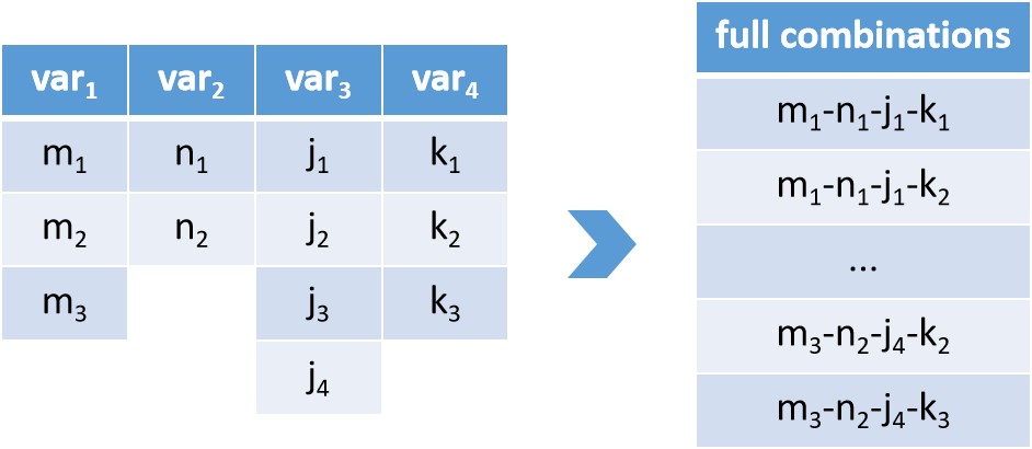
Figure 4.8 factors, levels and their full combinations

Nevertheless, it should be remembered that it is so tough for experiment that traverse all possible combinations (full factorial design) with the increasing number of factors in practice. From a certain dataset with indexing, it is not difficult to construct how many factors and corresponding levels it has, but not all possible combinations have been implemented, on the other hand.

4.2.3.3. Rearranged pseudo-tensor

Up to now, we consider all factors equally. However, the factors are mostly mix of the dependent and independent variables, or that of the experimental conditions and labels. They are intrinsically of different attributes. Sometimes, we might desire the model trained from our data set that can be distinguishable for some factors, simultaneously vary less for the others.

To fulfill that attributes of factors, a data structure called rearranged pseudo-tensor is introduced hereby (see Figure 4.9). In analogy with the concept of in chemistry, it attributes factors with active/inert type. For active type, full combinations of levels of that factors are arranged vertically. Similarly, inert ones are horizontally arranged. For each specific combinations of inert multiplied active factors, if there exists repeats, those data will be stacked in the 3rd dimension, namely the sampling axis, then forms different columns as showed in Figure 4.9 (empty column for no data in that combination of levels of factors).

Thus, maybe based on some priori things, we can artificially reorganize the data as this form for further investigation. Therefore for a certain design matrix with factorisable indexes, each column in it can be folded as the form of that pseudo-tensor. By applying statistical approach-designed aggregation function (see the next subsection Priori scoring), it is handy to measure then score how well that dimension matches the hypothesis.

Note

An aggregation function is a type of mapping from any set of numeric to scalar. The set of numeric can be a series, a vector, a tensor, or a customized structure such as the pseudo-tensor proposed in this section (e.g. mean, standard deviation, or etc.).

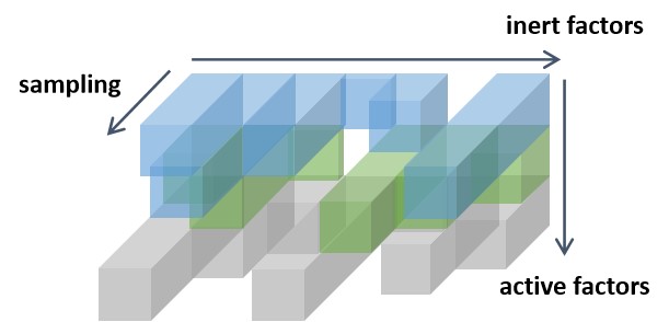
Figure 4.9 pseudo-tensor rearranged by respectively inert and active factors

Note that the prefix pseudo is due to that the length of dimension for sampling is not fixed in most cases (compared to conventional tensor with fixed lengths for respective dimensions). Moreover, with the increase of number of combinations among factors to be investigated, more columns in that tensor are tempt to be empty. Thus, the properties of unfixed-dimension, as well as sparsity of that data construction should be taken into consideration when we customize the aggregation function for scoring it.

4.2.3.4. Priori scoring

For quantification for what extent the data in certain dimension matches our priori, here devises an algorithm called priori scoring. Priori scoring is the default aggregation function to calculate the rearranged pseudo-tensor to a scalar. It mainly consists of two statistical components:

4.2.3.4.1. Normality statistic

For each column in the pseudo-tensor, its levels for all factors are of the same. Namely the data in the same column are sampled under the identical conditions. According to central-limit theorem, it guarantees the data within certain column will converge into normal distribution with probability. Causally the objective of the current statistic must be capable to summarize: a) basic location for numeric; b) the extent for the data biased from a normal distribution.

Priori scoring utilizes Shapiro-Wilk test to measure the normality, as showed in Figure 4.10. As from Shapiro-Wilk test, its statistic \(s_{sw}\) and \(p\)-value (\(p_{sw}\)) both vary from 0 to 1, the normality statistic of priori scoring \(s_{ps}\) takes the complex number space. For the data in a certain column, the Euclidean norm of \(s_{ps}\) is sample mean \(\bar{x}\); the direction of \(s_{ps}\) is determined by \(s_{sw}\) and \(1-p_{sw}\).

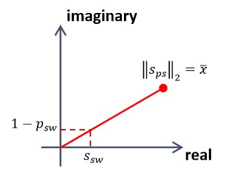
Figure 4.10 normality statistic of priori scoring

This design naturally satisfies aforementioned two requirements. For the data set with 0 variation (all equal), the \(s_{sw}\) and \(p_{sw}\) will simultaneously be 1. So it is absolutely reliable for the \(\bar{x}\) since the real component of \(s_{ps}\) is equal to \(\bar{x}\). As the data varies largely but with the same \(\bar{x}\), the \(s_{sw}\) vary not too much (comparatively high value) but \(p_{sw}\) will decrease. Under this circumstance, the real component of \(s_{ps}\) decrease correspondingly. If the data barely distributed as normality, then the \(p_{sw}\) will be considerably low. Therefore as the increase of imaginary component of \(s_{ps}\), the projection of \(s_{ps}\) in real axis will decrease further.

4.2.3.4.2. Variation statistic

For a certain rearranged pseudo-tensor consisted of multiple columns, applying aforementioned normality statistics can result in a complex matrix, likely with empty values. For simplification, we attribute the term group, for the combinations of levels among active factors.

Previous discussion reveals the real component of normality statistic is an effective indicator for summarizing the value as well as the distribution of the data under the identical conditions. Consider the pseudo-tensor: for each group, their combinations of levels among inert factors (horizontal arrangement) are of the same. Namely statistics within all groups vary almost equally in the sight of inert factors, which satisfies homoscedasticity of ANOVA test.

Suppose \(\boldsymbol{S} \in \mathbb{C}^{d_1 \times d_2}\) is the complex matrix obtained from pseudo-tensor after normality statistics. \(\boldsymbol{S}^\ast\) is the conjugate of \(\boldsymbol{S}\). Its projection on real axis \(\boldsymbol{P} \in \mathbb{R}^{d_1 \times d_2}\) can be calculated as:

(4.1)\[\boldsymbol{P} = \frac{1}{2} (\boldsymbol{S}+\boldsymbol{S}^\ast)\]

After dealing with the empty values (usually omitting), the variation of \(\boldsymbol{P}\) among and within groups is implemented via one-way ANOVA. Assume \(p_{ow}\) denotes the \(p\)-value of one-way ANOVA for some case, its final score \(e_{ps}\) evaluated by priori scoring algorithm is determined through the negative logarithmic space as:

(4.2)\[{e}_{ps} = -\text{log}({p}_{ow})\]

Therefore the higher the score of variation statistic, the higher tendency of variation among groups over that of within group ones, as well as the higher in probability that case matches the active/inert factors hypothesis.

4.2.3.4.3. Framework of algorithm

If we use \(\mathrm{T}^+\) to denote the rearranged pseudo-tensor. Consider a data set denoted as a design matrix \(\boldsymbol{D} \in \mathbb{R}^{n \times m}\). \(\boldsymbol{c}\) is the constructor consists of factors and corresponding levels for its all factorisable indexing. If \(k\) factors is assigned as \(\mathrm{F} = \{\boldsymbol{k}_1, \dots, \boldsymbol{k}_x\}\), a partitioning \(\{\mathrm{P}, \mathrm{P}^\prime\}\) for \(\mathrm{F}\) where \(\mathrm{P}\) is the set of active factors, and \(\mathrm{P}^\prime\) is the inert ones, is also required before calculation.

With \(\boldsymbol{D}\), \(\boldsymbol{c}\) and \(\{\mathrm{P}, \mathrm{P}^\prime\}\), the priori scoring algorithm can be summarized as the Table 4.2:

Table 4.2 framework of priori scoring algorithm

priori scoring algorithm
Requires: \(\boldsymbol{D}\), \(\boldsymbol{c}\), \(\mathrm{P}\) or \(\mathrm{P}^\prime\)
Export: evaluated scores \(\{e_1, e_2, \dots, e_m\}\)
for i in \(\{1, 2, \dots, m\}\): fold \(D_{:, i}\) to \(\mathrm{T}_{i}^+\) via \(f_1(D_{:, i}, \boldsymbol{c}, \mathrm{P})\) calculate \(\boldsymbol{S}_{i}\) and \(\boldsymbol{S}_{i}^\ast\) through normality statistic \(f_2(\mathrm{T}_{i}^+)\) obtain real projection matrix \(\mathrm{P}_{i}\) from \(0.5(\boldsymbol{S}_{i}+\boldsymbol{S}_{i}^\ast)\) from variation statistic \(f_3(\mathrm{P}_i)\) calculate \(p\)-value \(p_{i}\), with logarithmic space obtain its final score \(e_i\) return \(\{e_1, e_2, \dots, e_m\}\)

After which the evaluated scores \(\boldsymbol{e} \in \mathbb{R}^{+m}\) for \(\boldsymbol{D} \in \mathbb{R}^{n \times m}\) will be calculated. The significance ranking levels for all of those dimensions in priori scoring are determined using intervals with length of 10, from 0 to ceil of \(10 \cdot f_{\mathrm{ceil}} (0.1 \cdot e_{\mathrm{max}})\).

---

Authors:

Chen Zhang

Version:

0.0.5

Created on:

May 24, 2023