4.3.2. Anomaly and change

In the realm of data analysis, anomaly and change detection play pivotal roles in understanding the behavior of complex systems. Particularly in dynamic environments, where data patterns and distributions constantly shift, effective anomaly and change detection becomes crucial techniques and methodologies employed for identifying unusual patterns and significant variations in datasets.

Anomaly detection aims to identify observations that significantly deviate from the expected patterns or the main distribution of the data. By employing statistical algorithms, detected outliers can be indicative of errors, novelties, or can provide valuable insight into the underlying system. Change detection, on the other hand, focuses on identifying significant changes in the statistical properties or patterns of data over time. Such changes might indicate system failures, external disturbances, or natural evolution of the system. Change detection techniques range from simple threshold-based approaches to complex statistical tests and machine learning models, depending on the nature and complexity of the data.

4.3.2.1. Anomaly detection

The application scopes of anomaly detection, is usually confused from that of binary classification. In fact, many failures of algorithm in practical tasks are results from the lack of comprehension for the data self, as well as oversimplification for feature engineering. We mentioned what does pattern means in data, in aspect of binary classification task, its precondition for using is that we supposes two groups of datasets have their respective patterns, and their representations are possibly clustered in high dimension space individually.

To concrete this abstract concept, imagine two thought experiments: training classifiers for distinguishing images of cat and dog, and for distinguishing images of cat and no cat. For the former, obviously you know what those two species look like, but for the later, can you image a precise definition for the class no cat? A dog can be no cat, however a book, a pen, a cup can also be called no cat. Either cat or dog, is narrow concept with explicit definition, abstraction for these narrow concepts is also the suggested scope for practice of current AI approaches. But for no cat, it is a comparatively broader concept more than a clear definition.

Thus, for summary using the following Figure 4.25, the most difference between binary classification and anomaly determination, is that for binary classification, it actually calculates the most possible margin between two clusters, however for anomaly determination, it only hypotheses the existence of one cluster, then using certain approaches to determine the boundary of this cluster.

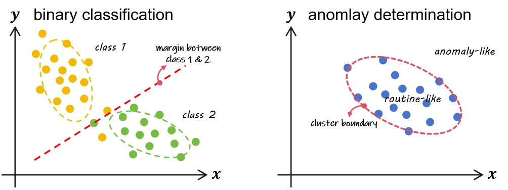
Figure 4.25 difference between binary classification and anomaly determination

Make confusion on those two types of tasks seems ridiculous, but this mistake takes place over and over on many junior data analysts. They uses classification algorithm frames to train models expected to make distinguishing on stable and unstable signals, on healthy and unhealthy cases, or such like. They integrated expertise, struggled in dealing with data cleaning and labeling, trained and validated the models. Nevertheless, once observations, with new patterns in comparison to the ones embedded in their training data, appear, the performance of the models decline, hence new model is in urgent. All things happen just like in an infinite loop.

Therefore, the correct understanding and definition of the problem is a prerequisite and crucial step in problem-solving. If our analytical data tends to establish one side pattern, various methods of anomaly detection will excel in such tasks.

4.3.2.1.1. Hotelling T-squared

The Hotelling T² statistic is a multivariate extension of the t-test. It is derived by Harold Hotelling in 1931 to deal with evaluating significance of mean differences between two or more groups of datasets containing multiple variables ([Ramirez1991, Holst2011]).

Criterion distribution is established using multivariate gaussian \(\mathcal{N}(\hat{\boldsymbol{\mu}}, \hat{\boldsymbol{\Sigma}}^{-1})\) where the parameter \(\hat{\boldsymbol{\mu}}\) and \(\hat{\boldsymbol{\Sigma}}^{-1}\) are unbiased estimations of mean vector and precision matrix using training data. For new observation \(\boldsymbol{x}^\prime\), define its T² statistic as:

(4.94)\[T^2 = \frac{N-M}{(N+1)M} (\boldsymbol{x}^\prime - \hat{\boldsymbol{\mu}})^\top \hat{\boldsymbol{\Sigma}}^{-1} (\boldsymbol{x}^\prime - \hat{\boldsymbol{\mu}}) \sim \mathcal{F}(M, N-M)\]

Note

Bias is a concept in parameter estimation in statistics. An essential hypothesis is that we always get samples rather than population as our dataset, however we generally want to make some conclusions on population via these samples. An identical statistic may differ on population and samples. It called bias in terminology. The unbiased estimation is designed in consideration of those impacts in order to reduce the bias of samples from population. (e.g. for \(n\) observations, if they are of population, the denominator of its standard deviation is \(n\), while if they are of samples from certain population, this value will be \(n-1\))

Where \(N\) is the number of observations, and \(M\) is the dimensionality. Now consider the condition \(N \geq M\) which can be easily achieved through data preparation or dimension reduction, the full rank property of \(\boldsymbol{\Sigma}\) can be established. Thus, the item of \((\boldsymbol{x}^\prime - \hat{\boldsymbol{\mu}})^\top \hat{\boldsymbol{\Sigma}}^{-1} (\boldsymbol{x}^\prime - \hat{\boldsymbol{\mu}})\) in Equation 4.94 is actually the sum of squares with \(M\) degree of freedom.

For new variable \(z\) as function of \(z = f(\boldsymbol{x}) \in \mathbb{R}^1\), the Jacobian transformation is generally used for calculation for its probability mass or density. In this case, the \(M\)-variate version of probability density function can be noted as:

(4.95)\[q(z) = \int_{-\infty}^{\infty} d\boldsymbol{x} \delta (z-f(x^{(1)}, \dots, x^{(M)})) p(x_1, \dots, x_M)\]

Where \(\delta\) is Dirac’s delta function. Now we assume there is \(M\) samples independently derived from \(\mathcal{N}(0, \sigma^2)\) noted as \(x_1, \dots, x_M\), and a coefficient \(c > 0\), the probability density function of variable \(u = c(x_1^2 + x_2^2 + \cdots + x_M^2)\) is:

(4.96)\[q(u) = \int_{-\infty}^{\infty} dx_1 \cdots dx_M \delta (u - c(x_1^2 + \cdots + x_M^2)) \prod_{n=1}^M \mathcal{N} (x_n | 0, \sigma^2)\]

It can utilize the \(M\)-dimensional spherical coordinates to make simplification for Equation 4.96, the infinitesimal of \(dx_1 \cdots dx_M\) can be equivalently replaced by the \(dr \cdot r^{M-1}dS_M\) (\(dr\) and \(r^{M-1}dS_M\) are infinitesimals of thickness, and surface area in \(M\)-dimensional sphere respectively). Let \(v = cr^2 = c \sum_{i=1}^{M} x_i^2\), \(dr\) will be \(d(v/c)^{1/2} = (1/2c) \cdot (v/c)^{(1/2)} dv\), the Equation 4.96 will be:

(4.97)\[q(u) = \int_{0}^{\infty} \frac{dv}{2c} (\frac{v}{c})^{(M/2)-1} \delta (u-v) \frac{1}{(2 \pi \sigma^2)^{M/2}} \exp(-\frac{v}{2c\sigma^2}) \int dS_M\]

For the last item \(\int dS_M\), it is the surface area of \(M\)-dimensional sphere with \(r = 1\). Consider the property of high dimensional sphere. \(\int S_M\) is actually \((2\pi^{M/2})/\Gamma(M/2)\).

As for a continuous function \(f(x)\), consider the symmetric property of \(\delta\) function, the variable change relationship can be established through the \(\delta\) functions as following:

(4.98)\[\int dx \delta (x - b) f(x) = \int dx \delta (b - x) f(x) = f(b)\]

Therefore the Equation 4.97 can be finally simplified as Equation 4.101:

Note

For a \(K\)-dimensional sphere with radius of \(r\), its volume is:

(4.99)\[V_K = \frac{\pi^{\frac{K}{2}}}{\Gamma(\frac{K}{2}+1)} r^K\]

Its surface area will be one dimension degenerated as the form of:

(4.100)\[S_{K-1} = \frac{2 \pi^{\frac{K}{2}}}{\Gamma(\frac{K}{2})} r^{K-1}\]

(4.101)\[\begin{split}q(u) &= \int_0^{\infty} dv \delta (u-v) \frac{1}{2c} (\frac{v}{c})^{\frac{M}{2}-1} (2 \pi \sigma^2)^{-\frac{M}{2}} \exp (-\frac{v}{2 c \sigma^2}) \frac{2 \pi^{\frac{M}{2}}}{\Gamma(M/2)} \\ &= \int_0^{\infty} dv \delta (u-v) \frac{1}{2 c \sigma^2 \Gamma(M/2)} (\frac{v}{2 c \sigma^2})^{\frac{M}{2}-1} \exp (-\frac{v}{2 c \sigma^2}) \\ &= \frac{1}{2 c \sigma^2 \Gamma(M/2)} (\frac{u}{2 c \sigma^2})^{\frac{M}{2}-1} \exp (-\frac{u}{2 c \sigma^2}) \sim \chi^2 (u | M, c \sigma^2)\end{split}\]

Here deduced the most important property: the probability density of sum of squares, is come from a certain \(\chi^2\) distribution with \(M\) degrees of freedom, and \(c \sigma^2\) as scale. For the item \((\boldsymbol{x}^\prime - \hat{\boldsymbol{\mu}})^\top \hat{\boldsymbol{\Sigma}}^{-1} (\boldsymbol{x}^\prime - \hat{\boldsymbol{\mu}})\), it uses unbias estimation as standardization while no spatial rescaling for \(\boldsymbol{x}^\prime\), thus \(c = \sigma^2 = 1\). Therefore, the final anomaly threshold is determined through the maximum likelihood estimation of \(\chi^2 (x | M, 1)\).

4.3.2.1.2. Empirical distribution and neighbors

In spite of concision and lightweight, Hotelling T² sometime shows insufficient accuracy due to its strong assumption on statistical distribution. Once the collected data is not as sufficient to satisfy the underlying conditions like \(F\) or \(\chi^2\) distributions, this method hits possible the ceiling.

Here introduce a non-parametric concept of empirical distribution which is defined as:

(4.102)\[p_{\mathrm{emp}} (\boldsymbol{x} | \boldsymbol{x}^{(1)}, \dots, \boldsymbol{x}^{(N)}) = \frac{1}{N} \sum_{n=1}^N \delta (\boldsymbol{x} - \boldsymbol{x}^{(n)})\]

It is a probability density function because for any \(\boldsymbol{x} \in \mathbb{R}^M\), its \(p_{\mathrm{emp}}\) value in Equation 4.102 is equal or greater than 1, while \(\int p_{\mathrm{emp}} d\boldsymbol{x} = 1\). For any point \(\boldsymbol{x}^\prime \in \mathbb{R}^M\), define its neighbor a \(M\)-dimensional sphere with radius \(\epsilon\), according to Equation 4.99 its volume will be \(V_M (\boldsymbol{x}^\prime, \epsilon) = (\epsilon^M \pi^{M/2}) / \Gamma(M/2 + 1) = C \cdot \epsilon^M\), where \(C\) is an \(\epsilon\) independent constant.

Therefore in empirical distribution, the probability of that \(\boldsymbol{x}^\prime\) will be \(p (\boldsymbol{x}^\prime) = k/(N \cdot V_M (\boldsymbol{x}^\prime, \epsilon))\), \(k\) is the number of existing data from \(x_1\) to \(x_N\) inside the \(V_M (\boldsymbol{x}^\prime, \epsilon))\) sphere. The anomaly statistic of \(\boldsymbol{x}^\prime\) is:

(4.103)\[a(\boldsymbol{x}^\prime) = - \ln p (\boldsymbol{x}^\prime) = - \ln k + M \ln \epsilon + C^\prime\]

Where \(C^\prime\) is a constant which independent with \(k\), and \(\epsilon\). The lower the \(k\) in condition of fixed \(\epsilon\), or the greater the \(\epsilon\) in condition of fixed \(k\), the less probability of \(\boldsymbol{x}^\prime\) as anomalous instance. It is not difficult to imagine, if we modeled a certain dataset \(D = \{\boldsymbol{x}_1, \dots, \boldsymbol{x}_N\}\) with almost normal observations, for given radius \(\epsilon\), the more similar data points distributed inside the \(V_M\) of a new observation, the higher tendency of no anomaly; while for given \(k\), if a new observation will require greater radius \(\epsilon\), it means the higher bias this new observation distributed from the original \(D\), so it is safe to say it, anomaly like.

We can also back the topic to binary classification. If we use \(y=0\) and \(y=1\) to label the classes of normal and anomaly, respectively, the anomaly statistic can be noted as:

(4.104)\[a (\boldsymbol{x}^\prime) = \ln \frac{p(\boldsymbol{x}^\prime | y=1, D)}{p(\boldsymbol{x}^\prime | y=0, D)}\]

Consider the bayes formula:

(4.105)\[p(\boldsymbol{x}^\prime|y=i, D) = \frac{p(y=i |\boldsymbol{x}^\prime, D) p(\boldsymbol{x}^\prime, D)}{p(y=i, D)} = \frac{N^i (\boldsymbol{x}^\prime)}{k} \cdot \frac{1}{\pi^i} \cdot p(\boldsymbol{x}^\prime, D)\]

The \(N^i (\boldsymbol{x}^\prime) / k\) corresponds to \(p (y=i | \boldsymbol{x}^\prime, D)\) that for \(k\) neighbors of \(\boldsymbol{x}^\prime\), the number of data points in \(D\) with label of \(y=i\); While the \(\pi^i\) corresponds to the fraction of \(y=i\) among total data points. Thus, the Equation 4.104 can be further simplified into:

(4.106)\[a (\boldsymbol{x}^\prime) = \ln \frac{\pi^0 N^1 (\boldsymbol{x}^\prime)}{\pi^1 N^0 (\boldsymbol{x}^\prime)}\]

For method using neighbor data points, it requires computing and sort the distance. The distance measure of neighbor related method is pre-determined. Customarily, people use Euclidean distance in original space (e.g. for \(\boldsymbol{a}\) and \(\boldsymbol{b}\), \(d^2 (\boldsymbol{a}, \boldsymbol{b}) = (\boldsymbol{a}-\boldsymbol{b})^\top(\boldsymbol{a}-\boldsymbol{b})\)). Or for some algorithm frames, the order of norm has also been designed as an optional callback for distance measurement. Whatever norm order was defined, the calculation of distance takes places in original Cartesian coordinate system.

Based on the former discussion, it is cleared how neighbors distributed makes difference on the accuracy of neighbor related method. Therefore, the performance ceil for this algorithm, depends seldom on norm order, it indeed relies on whether we can obtain a space, that data points with same labels can as clustered as possible, while ones with different labels can be separated. From previous section we know the matrix, or transformation means certain operation(s) on the original (Cartesian) space. Here we introduce the Riemannian metric, to fulfill that spatial transformation we desired.

Note

Figure 4.26 coffee mug as a homeomorphic object of donut [Hubbard2012]

When it comes to the concept homeomorphism in topology, a very famous example is the joke about donut and coffee mug [Hubbard2012]. As it is still little difficult to imagine, it is preferential to use decompression toy as analogous example: now there is an ideal elastic decompression toy, you can press, tense, twist, squeeze it into whatever shape you like. For this toy, although it can possess different shapes under varying effects of deformation, these shapes are of homeomorphic. While the operations of deformation, are conceptually in consistence with the transformation on the original space.

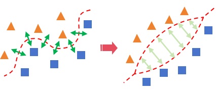
Figure 4.27 illustration for deformation in Riemannian geometry

The concept of homeomorphism is of essence to understand Riemannian metric. As illustration in Figure 4.27, transformation on Riemannian geometry allows local deformation anywhere. Imagine all of the data points located on surface of a certain Riemannian geometry (ideal elasticity), it can get any desired new distribution of these data points, by introducing a combination of certain local deformation operations.

The measure of distance varies from different algorithms. Euclidean defined as \(d^2 (\boldsymbol{a}, \boldsymbol{b}) = (\boldsymbol{a} - \boldsymbol{b})^\top\boldsymbol{I}(\boldsymbol{a} - \boldsymbol{b})\) can be deem as the computation in original Cartesian space, while the anomaly statistic mentioned in Hotelling T-squared is equivalent of using a rescaled Cartesian space via \(\hat{\boldsymbol{\Sigma}}^{-1}\). More generally, it can define a Riemannian space \(\boldsymbol{R}\) that the corresponding distance measure is \(d^2_{\boldsymbol{R}} (\boldsymbol{a}, \boldsymbol{b}) = (\boldsymbol{a} - \boldsymbol{b})^\top \boldsymbol{R} (\boldsymbol{a} - \boldsymbol{b})\). How to determine an optimal Riemannian metric \(\boldsymbol{R}\) so that data points with identical labels can be clustered, while different clusters can be as separated as possible (like the illustration in Figure 4.27), is the scope of a sub field in machine learning, called metric learning.

For more generic solution, we can discuss this problem in frame of multi classification so that it is rational to assume a prior weights for all categories, and the prior weight for peers of \(y = y^{(n)}\) is \(w_{(n)}\). Focus on a certain \(\boldsymbol{x}^{(n)}\) in Equation 4.102 with label \(y = y^{(n)}\), define the set \(N^{(n)}\) the points with identical label as \(\boldsymbol{x}^{(n)}\), among \(k\)-nearest neighbors of \(\boldsymbol{x}^{(n)}\), the mathematical expression for concept data points with identical labels can be clustered, can be represented as:

(4.107)\[\psi_1^{(n)} (\boldsymbol{R}) = \sum_{i \in N^{(n)}} d_{\boldsymbol{R}}^2 (\boldsymbol{x}^{(n)}, \boldsymbol{x}^{(i)})\]

While for the concept different clusters can be as separated as possible:

(4.108)\[\psi_2^{(n)} (\boldsymbol{R}) = \sum_{j \in N^{(n)}} \sum_{l=1}^N I_{y^{(l)} \neq y^{(n)}}(y^{(l)}) \left[ 1 + d^2_{\boldsymbol{R}} (\boldsymbol{x}^{(n)}, \boldsymbol{x}^{(j)}) - d^2_{\boldsymbol{R}} (\boldsymbol{x}^{(n)}, \boldsymbol{x}^{(l)}) \right]_{+}\]

The item \(\boldsymbol{x}^{(j)}\) and \(\boldsymbol{x}^{(l)}\) in Equation 4.108 are the data points, with and without identical label as \(\boldsymbol{x}^{(n)}\) respectively. Assume the set of labels \(C = {1, \dots, s}\) represents for \(s\) different classes, the optimization target of Riemannian \(\boldsymbol{R}\) is:

(4.109)\[\Psi (\boldsymbol{R}) = \frac{1}{N} \sum_{c=1}^s \sum_{n=1}^N \left[ w_c \cdot \psi_1^{(n)} (\boldsymbol{R}) + \sum_{m \in \{c\}^C} w_m \cdot \psi_2^{(n)} (\boldsymbol{R}) \right] \quad \mathrm{s.t.} \> \boldsymbol{R} \succeq 0\]

The constraint \(\boldsymbol{R} \succeq 0\) is for semi-positive definite matrix. Therefore set the eigen value(s) as 0, if negative value dimension(s) were calculated during learning steps. \(\{c\}^C\) is the complementary set of \(c\) in \(C\). Metric learning updates the \(\boldsymbol{R}\) using subgradient via the item \(\partial \Psi (\boldsymbol{R}) / \partial \boldsymbol{R}\) until convergence. Using decomposition on the updated Riemannian metric \(\boldsymbol{R}^* = \boldsymbol{L}^\top \boldsymbol{L}\), the distance measure in Riemannian space is therefore \((\boldsymbol{a} - \boldsymbol{b})^\top \boldsymbol{R}^* (\boldsymbol{a} - \boldsymbol{b}) = [\boldsymbol{L}(\boldsymbol{a} - \boldsymbol{b})]^\top [\boldsymbol{L}(\boldsymbol{a} - \boldsymbol{b})]\). Thus, the relationship between original space and the final Riemannian space is nothing other than the transformation \(\boldsymbol{L}\).

4.3.2.1.3. Bayesian and mixture Gaussian

text here

4.3.2.1.4. Directional data

The significance of introducing the concept of directional data, as well as its associated modeling methods, is primarily for aligning the dimensions of data from disharmonious ranges. For a simple instance, the word as counted for characterizing certain topic may varies from document carriers. In this circumstance, the utilization for Gaussian distribution will lose its rationality. In addition, the deduction for modeling directional data is conducted through the high-dimensional spherical representation in orthogonal coordinates. There is therefore the underlying established assumption for the directional data that the utilization of this approach would be of compact but effective representation to data, in the condition of irrelevance on dimension.

The Von Mises Fisher distribution as a parametric approach to the directional data, is constituted of the mean direction \(\boldsymbol{\mu}\) and the concentration parameter \(\kappa\). In the context of a \(M\)-dimensional space, its probability density function of parameters \(\boldsymbol{\mu}\) and \(\kappa\) is determined by:

(4.110)\[\mathcal{M}(\boldsymbol{x}|\boldsymbol{\mu}, \kappa) = \frac{\kappa^{M/2-1}}{(2\pi)^{M/2} I_{M/2-1} (\kappa)} \exp(\kappa \boldsymbol{\mu}^\top \boldsymbol{x})\]

Where \(\boldsymbol{\mu}\) is an \(M\)-length unit vector, and the item \(I_{M/2-1} (\kappa)\) refers to the modified Bessel function of the 1st kind. In general, a \(o\)-ordered 1st kind modified Bessel function \(I_o (x)\) is defined as:

(4.111)\[I_o (x) = \frac{2^{-o} x^{o}}{\sqrt{\pi} \Gamma (x + 0.5)} \int_0^{\pi} d\phi \cdot \sin^{2 o} \phi \exp (x \cos \phi)\]

We use the \(c_M (\kappa)\) to substitute the coefficient term for that of \(\exp\) in Equation 4.110. As for the data set \(D = \{ \boldsymbol{x}^{(1)}, \dots, \boldsymbol{x}^{(n)} \}\), its logarithmic Lagrange for the most likelihood estimation (MLE) on \(\boldsymbol{\mu}\) is:

(4.112)\[L (\boldsymbol{\mu}, \kappa | D) = \ln \prod_{n=1}^N c_M (\kappa) \exp (\kappa \boldsymbol{\mu}^\top \boldsymbol{x}^{(n)}) = \sum_{n=1}^N \{ \ln c_M (\kappa) + \kappa \boldsymbol{\mu}^\top \boldsymbol{x}^{(n)} \}\]

The partial differential of the generalized Lagrange of Equation 4.112 using the constraint of \(\boldsymbol{\mu}^\top \boldsymbol{\mu} = 1\) with coefficient \(\lambda\) is:

(4.113)\[\frac{\partial}{\partial \boldsymbol{\mu}} (L - \lambda \boldsymbol{\mu}^\top \boldsymbol{\mu}) = \kappa \sum_{n=1}^N \boldsymbol{x}^{(n)} - 2 \lambda \boldsymbol{\mu} = 0\]

Therefore the MLE on \(\hat{\boldsymbol{\mu}}\) is equal to \(\boldsymbol{s} / \sqrt{\boldsymbol{s}^\top \boldsymbol{s}}\) where the \(\boldsymbol{s}\) satisfies \(\boldsymbol{s} = ( \sum_{n=1}^N \boldsymbol{x}^{(n)} ) / N\). There is not explicit solution for analytically estimating the concentration parameter \(\kappa\) so far. For reference, Oinar et al. gave an intuitive demonstration for the 3-dimensional Von Mises Fisher distributions with different \(\kappa\), as showed in Figure 4.28. The lower the \(\kappa\), the more dispersive the data points are.

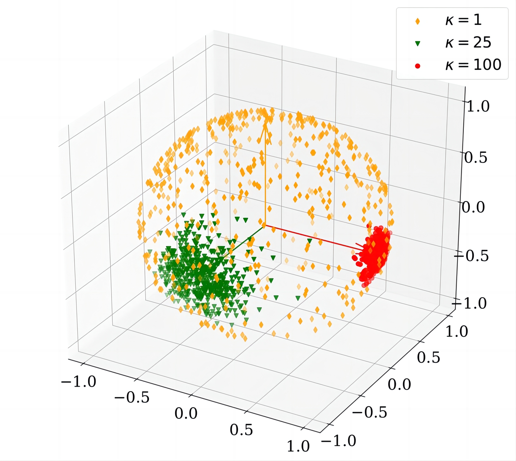
Figure 4.28 3-dimensional Von Mises Fisher distributions with varying \(\kappa\) [Oinar2023]

As for a new direction \(\boldsymbol{x}^\prime\), the measurement for the anomaly based on the Von Mises Fisher distribution can be defined using its negative logarithmic likelihood \(- \ln \mathcal{M} (\boldsymbol{x}^\prime | \boldsymbol{\hat{\mu}}, \kappa)\):

(4.114)\[\begin{split}a(\boldsymbol{x}^\prime) &= - \ln \{c_M (\kappa) \cdot \exp (\kappa \boldsymbol{\hat{\mu}}^\top \boldsymbol{x}^\prime)\} \\ &= - \ln \{c_M (\kappa) \cdot \frac{\exp(\kappa)}{\exp(\kappa)} \cdot \exp (\kappa \boldsymbol{\hat{\mu}}^\top\boldsymbol{x}^\prime)\} \\ &= C + \kappa - \kappa \boldsymbol{\hat{\mu}}^\top\boldsymbol{x}^\prime \propto 1 - \boldsymbol{\hat{\mu}}^\top \boldsymbol{x}^\prime\end{split}\]

Where \(C\) in Equation 4.114 refers to a \(\boldsymbol{x}^\prime\) irrelevant constant. Using the Equation 4.95 to change the variable of anomaly \(a\) as a function of \(1-\boldsymbol{\hat{\mu}}^\top \boldsymbol{x}^\prime\), the probability of \(a(\boldsymbol{x}^\prime)\) can be represented as:

(4.115)\[p(a) = \int_{S_{M}} d\boldsymbol{x} \delta(a - (1 - \boldsymbol{\hat{\mu}}^\top \boldsymbol{x})) c_M (\kappa) \exp(\kappa \boldsymbol{\hat{\mu}}^\top \boldsymbol{x})\]

\(S_M\) is the surface of a \(M\)-dimensional sphere. The \(d\boldsymbol{x}\) represents the differential area of \(S_M\). Consider the \(M\)-dimensional sphere is the integration of its \(M-1\)-dimensional spherical surface along the radian angle \(\theta\). The differential \(d\boldsymbol{x}\) can be represented by the \(d\theta \sin^{M-2}\theta dS_{M-1}\) (due to the differential \(dS_{M-1}\) is the function of \(r^{M-2}\), the \((r \cdot \sin \theta)^{M-2}\) can project the \(M-1\)-dimensional sphere on the radian angle \(\theta\), in unit sphere the \(r = 1\)).

As the \(\boldsymbol{\hat{\mu}}\) and \(\boldsymbol{x}\) in Equation 4.115 are both unit vectors, the relationship \(|\boldsymbol{\hat{\mu}}||\boldsymbol{x}| = 1\) can be established. The radian angle \(\theta\) can therefore be defined using the relationship \(\cos \theta = \boldsymbol{\hat{\mu}}^\top \boldsymbol{x}\). Ignore the \(a\) irrelevant terms, consider the property of \(\delta\) function as showed in Equation 4.98, the Equation 4.115 can be further simplified as:

(4.116)\[\begin{split}p(a) &\propto \int_{S_{M}} d\theta \sin^{M-2}\theta dS_{M-1} \delta (a-(1-\cos\theta)) \exp(\kappa\cos\theta) \\ &= \int_0^{\pi} d\cos\theta \cdot \delta (\cos\theta-(1-a)) \cdot (1-\cos^2\theta)^{\frac{M-3}{2}} \exp(\kappa \cos\theta) \int_{{S}_{M-1}} d{S}_{M-1} \\ &= (2a - a^2)^{\frac{M-3}{2}} \exp(\kappa-\kappa a)\end{split}\]

\(p(a)\) is the probability of anomaly therefore \(a \leq 1\) can be established. It is therefore rational to apply low-rank approximation, to ignore the term of \(a^2\). Consequently, the Equation 4.116 can further be simplified as proportional to \(a^{(M-1)/2-1}\exp(- \kappa a)\), which is exactly the kernel of \(\chi^2 (M-1, 0.5\kappa)\).

---

Authors:

Chen Zhang

Version:

0.0.5

Created on:

Apr 2, 2024