2.3.2. Adaptive AI with online learning

The architectural analysis of edge intelligence systems across domains mentioned in previous tutorial, from life-saving surgical robotics to ambient-aware smart homes, reveals a fundamental truth: true device autonomy hinges on an algorithm’s capacity for perpetual contextual adaptation. As established in our prior examination of streaming data ecosystems, edge devices operate in inherently nonstationary environments where sensor patterns, user behaviors, and operational constraints evolve continuously. This dynamism renders conventional static models obsolete, demanding instead AI systems that implement sustained environmental symbiosis through online learning mechanisms.

The critical differentiator lies not in hardware specifications, but in a model’s architectural capacity to organically assimilate streaming data. Successful edge intelligence implementations share a common DNA: machine learning architectures that treat data ingestion as a continuous calibration process rather than discrete training episodes.

2.3.2.1. Redefining intelligence via adaptive models

2.3.2.1.1. Breaking the infinite modeling cycle

While the term model remains ubiquitous in AI practice, practitioners often find themselves trapped in an infinite loop of model-design → deployment → concept drift → re-modeling. This Sisyphean cycle stems from treating models as fixed-parameter predictors frozen in temporal specificity. In edge intelligence contexts, successful implementations redefine models as continuously evolving entities - dynamic systems that self-calibrate through perpetual interaction with their operational environments.

2.3.2.1.2. Mathematical metaphors for adaptive systems

Effective edge AI mirrors how mathematicians distinguish between function families (e.g., quadratic functions) and specific implementations (e.g., y=2x²+3). Consider economic policymaking: while applying Shanghai’s income benchmarks to rural Gansu would fail, the underlying methodology of per-capita analysis remains sound. This reveals the core paradigm the edge AI implementations require:

• Meta-architectures providing methodological frameworks

• Contextual instantiation through localized data streams

• Bayesian adaptability enabling probabilistic adjustments

This approach transforms models from static equations into smart containers that maintain core analytical principles, dynamically adjust parameters like regulatory policies adapting to regional economies, and preserve computational efficiency through selective updates.

2.3.2.2. Self evolving meta models and demonstrations

2.3.2.2.1. Home blood pressure monitor

Here we contextualize the Code 2.24 on an edged blood pressure tracking system. The following implementation embodies the core principles of edge AI adaptability through a Bayesian meta-container architecture designed for multi-parameter health monitoring. This self-evolving system demonstrates how medical diagnostic devices can maintain operational relevance amidst gradual physiological shifts.

Code 2.27 dynamic bayesian blood pressure tracking system

from info.me import bayes as bys
from scipy import stats as st
from queue import Queue
import numpy as np

avg_dbp, avg_sbp, avg_pr = 73, 109, 87
avg_mean = np.array([avg_dbp, avg_sbp, avg_pr])
init_dis = st.multivariate_normal(avg_mean, np.eye(len(avg_mean)))
meta, container = bys.gaussian(kernel=init_dis), Queue()
shift_dis = st.multivariate_normal(avg_mean + np.array([-5, 4, 5]), np.eye(len(avg_mean)))  # data shift simulator
_ = [container.put(shift_dis.rvs(30)) for _ in range(10)]

while not container.empty():
    meta.update_posterior(posterior=container.get())

print(meta.conjugate.mean)
# [ 67.81901927 112.61276238  91.71077485], may vary

In the Code 2.27 we assumed the independence hypothesis among variable avg_dbp, avg_sbp, and avg_pr for simplification; If any canonical knowledge is accessible (e.g., WHO standards), their correlation, as prior knowledge, can also be embedded inside when a Bayesian container is initialized (the highlighted line in Code 2.27).

2.3.2.2.2. Individualized treatment program

Edge intelligence demonstrates universal applicability in personalized treatment regimens either. The Code 2.28 illustrates how Bayesian solvers enable dynamic tracking and evaluation throughout radiation therapy. While static models trained on big data may establish general priors like the generic_prior, clinical implementation must address individual variations in patients’ responses to radiation doses. This case study implements a Bayesian pharmacokinetic framework that initializes with generic physiological priors, then continuously adapts through dynamic updates based on real-time biomarkers. The critical challenge lies in precisely quantifying these inter-patient variations and optimizing phased treatment plans accordingly. By assimilating observed therapeutic responses, including tumor regression rates and marrow toxicity events, the system transforms fixed protocols into adaptive therapeutic trajectories, exemplifying contextual symbiosis between AI and clinical workflows.

Code 2.28 pharmacokinetic model for precision radiotherapy

from scipy import stats as st
from info.me import bayes as bys


generic_prior = {'k_tumor': 0.05, 'k_marrow': 0.02,
                 'beta_t': st.gamma(2.00, 2.00), 'beta_m': st.gamma(1.50, 3.33)}
bys_tumor = bys.poisson(kernel=st.poisson(1.0), prior=generic_prior['beta_t'])
bys_toxicity = bys.poisson(kernel=st.poisson(1.0), prior=generic_prior['beta_m'])
beta_est = (lambda obs, dose, eff: round(obs / (dose * eff)))
patient = [(3.7, 15, 2), (5.0, 25, 5), (6.2, 4, 18), ]  # 3 times radiotherapy, [dose, tumor_kill, marrow_kill]

for dose_gbq, tumor_event, tox_event in patient:
    bys_tumor.update_posterior(posterior=np.array([beta_est(tumor_event, dose_gbq, generic_prior['k_tumor']), ]))
    bys_toxicity.update_posterior(posterior=np.array([beta_est(tox_event, dose_gbq, generic_prior['k_marrow']), ]))
    ...  # visualization code for updated distributions here

The implementation of the pharmacokinetic framework above reveals critical dynamics through the Figure 2.20. Figure 2.20 (a) demonstrates leftward shifting of \(\beta_t\) posterior distribution after the final update, indicating increased tumor radiation resistance. Tracking initial priors and post-treatment sensitivities in Figure 2.20 (b) reveals concurrent elevation of marrow tissue vulnerability as tumor sensitivity declines. Following the second treatment, Bayesian predictive distributions for varying dose levels (Figure 2.20 (c)) suggest a safe therapeutic window of 5.05-6.50 GBq when constrained by clinical thresholds (≥10 tumor kill events with ≤3 marrow toxicity events). Selecting 6.20 GBq enables probabilistic projections of therapeutic outcomes through dose-specific PMF visualizations (Figure 2.20 (d)). Subsequent posterior updates after phase advancement (Figure 2.20 (e)) expose diminishing returns: the overlapping region satisfying clinical constraints virtually disappears, suggesting limited therapeutic benefit from continued radiotherapy. This adaptive quantification prompts consideration of alternative treatment modalities.

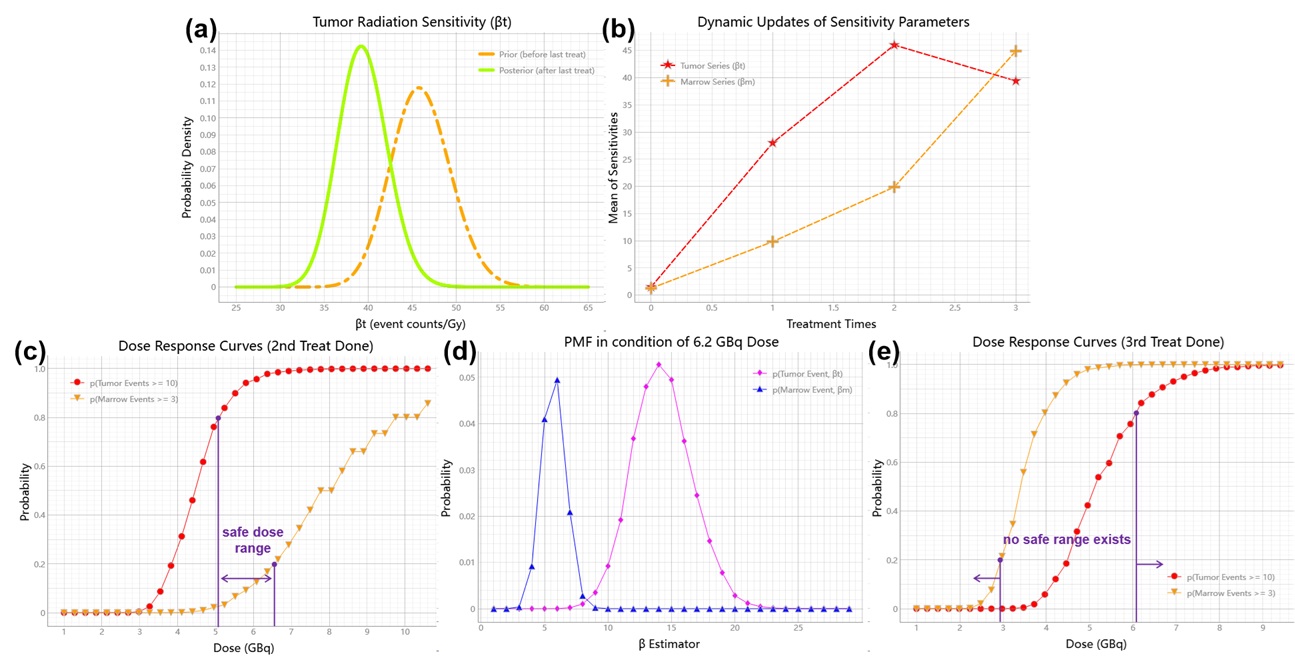
Figure 2.20 Bayesian precision radiotherapy

The dynamic nature of adaptive AI introduces real-time evaluation mechanisms during treatment, providing critical references for clinical decision-making. In this case, repeated therapies led to significant shifts in tumor and marrow responses to radiation, challenging the safety and efficacy of conventional radiotherapy. This necessitates a more cautious reassessment of therapeutic trade-offs.

2.3.2.2.3. Personalized adaptive image segmentation

Edge medical imaging requires models to self-evolve with anatomical drift. Static segmentation architectures fail to track time-dependent tissue variability across patients. Meta U-Net implementations achieve embedded evolution through dynamic filter calibration continuously adjusting convolutional components using on-device imaging streams. This enables medical segmentation pipelines to maintain precision as organ morphology shifts, exemplifying edge intelligence’s core principle: models as living systems, not frozen artifacts. The Code 2.29 concretes the edge meta AI architecture Code 2.25 in medical segmentation model training for patient personalization.

Code 2.29 self adaption U-Net for image segmentation

from info.net import unet
import os


patient_imgs, patient_segs = ..., ...  # list[img_or_seg_path], pairwise
model = unet(mirror_channels=[8, 16, 32], in_dimension=3) if not os.path.exists(_m := 'patient_seg') else load(_m)
while True:

    ...  # some AI-assistant application here

    if device.in_idle():
        with model.infer_session() as md:
            dice = md.score(train=(img_loader(_) for _ in patient_imgs),
                            target=(img_loader(_) for _ in patient_segs))
        if dice > thre:
            with model.train_session() as md:
                md.solve(train=(img_loader(_) for _ in patient_imgs),
                         target=(img_loader(_) for _ in patient_segs),
                         stop_conditions={'loss': thre})

This self-adaptive architecture demonstrates how edge-native online learning mechanisms transform static models into computational organisms. By selectively activating parameter updates during device idle cycles, the system achieves two symbiotic objectives: (1) real-time adaptation to anatomical shifts through dynamic filter recalibration, while (2) preserving computational resources via threshold-controlled training triggers. The dice > thre condition embodies edge intelligence’s essential trade-off: evolving only when environmental changes threaten operational validity. Such implementations prove that medical AI need not choose between generalization and personalization when models architecturally embrace perpetual metamorphosis.

---

Authors:

Chen Zhang

Version:

0.0.6

Created on:

May 10, 2025